Abstract
Free full text

Coronary vessel trees from 3D imagery: A topological approach
Abstract
We propose a simple method for reconstructing vascular trees from 3D images. Our algorithm extracts persistent maxima of the intensity on all axis-aligned 2D slices of the input image. The maxima concentrate along 1D intensity ridges, in particular along blood vessels. We build a forest connecting the persistent maxima with short edges. The forest tends to approximate the blood vessels present in the image, but also contains numerous spurious features and often fails to connect segments belonging to one vessel in low contrast areas. We improve the forest by applying simple geometric filters that trim short branches, fill gaps in blood vessels and remove spurious branches from the vascular tree to be extracted. Experiments show that our technique can be applied to extract coronary trees from heart CT scans.
1. Introduction
According to the US center for disease control and prevention data, heart disease is the first leading cause of death in the USA (National Center for Health Statistics, 2004). Segmentation of coronary trees from chest computed tomography (CT) scans is an important step toward early detection of plaques, aneurysms, stenoses and abnormal configurations of coronary arteries which could potentially lead to heart failure. Even though visual inspection of 2D slices is currently the most common way of making diagnosis based on cardiac CT scans, reliable segmentation of 3D models of coronary arteries from 3D imagery could eventually make the process less labor-intensive by helping radiologists to correlate the information from different slices or to simulate imaging techniques they are most familiar with (like angiography). The ability to extract 3D structures could also help to co-register different images, possibly captured as different times or using different methods, like CT, magnetic resonance imaging (MRI) or X-ray angiography.
In this paper, we propose a simple algorithm that can be used to reconstruct vascular trees from 3D images. This is known to be a challenging problem because of imperfections of the data such as noise, varying intensity of similar tissue and varying contrast. We deal with these challenges by employing discrete topological tools. One of the goals of discrete topology is finding and describing persistent features that cannot be removed by small perturbations of the data. We use persistence to filter out unimportant features that result from noise present in the data.
The structure of the paper is as follows. First, (Section 2) we discuss the related work on blood vessel segmentation. In Sections 3 and 4 we describe the two major stages of our algorithm: computing the set of persistent maxima on 2D slices through the data and reconstruction of blood vessel trees from those persistent maxima. Experimental results obtained for clinical datasets are discussed in Section 5. Finally, we discuss future research directions in Section 6.
2. Prior work
Blood vessel extraction algorithms have been receiving significant amount of attention in recent years (overviews of the subject can be found in Kirbas and Quek, 2004; Bühler et al., 2002; Felkel et al, 2001). We discuss the approaches related to the one presented in this paper below.
Ridge-based approaches view blood vessels as intensity ridges in the image and focus on extracting a representation (most frequently, a graph representation) of the ridges. Ridges define an approximation of the vessel skeletons or centerlines. The algorithm introduced in this paper is a ridge-based algorithm: it generates points that tend to be densely distributed along ridges and uses this set of points as a basis for vessel reconstruction.
An approach that allows one to trace a vessel centerline as well as estimate the width of the vessel at every point of the centerline is described in Aylward et al. (1996) and Aylward and Bullitt (2002). The method works by first projecting the user-specified seed point to a nearby ridge and then following that ridge. The direction of the vessel is estimated based on Hessians of the intensity function computed on different scales (the mathematical principles of this process as well as its robustness with respect to noise are discussed in Pizer et al., 1998). The scale is related to the width of the vessel that is being reconstructed and can be dynamically updated during the process. Other approaches based on tracking or optimizing the centerline either from one or between two user-specified points are discussed in Wesarg and Firle (2004), Wink et al. (2000) and Kanitsar et al. (2001).
Similar to the algorithm discussed in this paper, the one described in Florin et al. (2004) also generates a set of sample points near the centerlines of blood vessels and then connects them using the MST algorithm. However, there is a substantial difference in how the sample points are generated. In Florin et al. (2004), they are found as intensity maxima along rays entering the heart transversally. The maxima are examined for a number of properties (intensity range, peak shape, distance from the heart wall) to discard some of the false positives. Samples obtained this way can generally be located anywhere inside the vessels, so they are improved using eigenvalue analysis motivated by Krissian et al. (1998). In order to ensure dense distribution of samples along the blood vessels, a vessel tracking algorithm is used to follow the vessels locally and place more samples along them. We think that our way of generating samples on the vessels as maxima on 2D slices rather than rays is more natural. Our algorithm is also simpler to implement, in particular it does not require initial heart segmentation or analysis of the peak shape to work (although both could be considered as a way to reduce the number of false positives in our approach).
The algorithm introduced in Yim et al. (2000) uses intensity-driven region-growing to represent the image as a directed tree. The tree is then cleaned up based on user interaction or by applying a procedure similar to the forest trimming operation that we use in this paper. The directed tree representation of Yim et al. (2000) uses all voxels as the vertices, while we first select voxels that are likely to be on the vessels and then connect them into a forest based only on their distribution in 3D. Discarding the intensity information before the tree building stage leads to a procedure that could in some cases be more robust with respect to noise and intensity variation along a vessel. In particular, contrary to Yim et al. (2000), we do not need to compare the intensities of voxels that are far away in the image when building the forest. Such comparisons may lead to incorrect tree growing order when intensity is nonuniform along a vessel.
The algorithm of Deschamps and Cohen (2001), first generates an incomplete reconstruction of a blood vessel by thresholding the vesselness measure of Frangi et al. (1998). Then, the connected components of the incomplete reconstruction are joined using paths minimal with respect to a potential function defined using the vesselness measure. The robust maxima used to build the vessel trees in our algorithm may be thought of as a counterpart of the incomplete reconstruction. However, our way of connecting them to form vessel trees is based purely on their proximity information, while Deschamps and Cohen (2001) uses a more complicated method based on minimal paths with respect to a potential based on the vesselness measure. The vesselness measure can potentially be used to reduce the number of sample points generated by our algorithm (see discussion in Section 6).
Although our algorithm is based on different principles, we view it as a potential complement of approaches based on deformable models (Kass et al., 1988; McInerney and Terzopoulos, 1996; Sethian, 1999). The trees obtained using the procedure described in this paper could be used to obtain initial conditions or additional constraints for these methods, possibly improving their efficiency, convergence as well as the segmentation results. Adaptations of deformable model techniques to the problem of blood vessel segmentation are discussed in Frangi et al. (1999), Bulpitt (1998), McInerney and Terzopoulos (1999), Yim et al., 2001, Lorigo et al. (2000), Deschamps and Cohen (2002) and Nain et al. (2004). Similarly, statistical techniques such as those used in Chung et al. (2002, 2004) may be used to classify pixels near the coronary tree computed using our algorithm, providing information about the geometry of the artery (e.g., allowing one to detect stenosis) or about plaque buildup. Such applications will be explored in future work.
3. Computing persistent maxima
The purpose of this step is to generate points near the centerlines of blood vessels. Blood vessels have larger intensity than the surrounding tissue and are essentially 1D structures. Therefore, a blood vessel that intersects a 2D slice through the input data produces a local maximum of intensity on the slice near the intersection point. The converse is generally not true because of noise and presence of other features: there are several local maxima that do not correspond to blood vessels (Fig. 1). In fact, noise makes the distribution of the local maxima rather unstructured. We deal with this problem by filtering out the ‘weak’ local maxima using persistence (Edelsbrunner et al., 2001). This allows to reject local maxima due to noise while mostly preserving the ones defined by blood vessels. Our algorithm computes such local maxima on all axis-oriented 2D slices through the input volume. By an axis-oriented slice we mean a slice perpendicular to one of the coordinate axes. Persistent local maxima tend to be aligned with the blood vessels, as shown in Fig. 2.
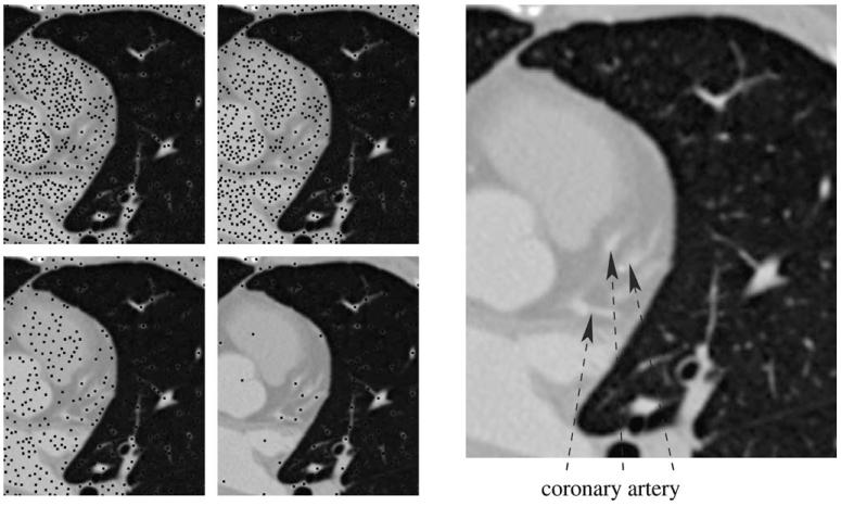
Left: maxima (black dots) of persistence 0 and 160 (top row) and 640 and 2560 (bottom row) in a slice through one of the sample datasets. The voxel intensities range from 0 to 65535. The last persistence threshold is the most suitable for use in our algorithm. Right: high intensity regions corresponding to the coronary artery.
Persistence of a local maximum x0 of a continuous function f can be formally defined as a maximum positive number p for which there are no points with value larger than f(x0) in the set L(x0;p), defined as the connected component of {x|f(x) > f(x0) − p} containing x0. Intuitively, persistence can be thought of as a relative measure of height of a local maximum. If a local maximum has persistence greater than p then it cannot be ‘removed’ by perturbing the function by less than p/2 (such a perturbation can increase or decrease a value by no more than p/2 and therefore is able to alter relative height of a maximum by up to p): in any perturbed function there is a local maximum in L(x0;p) (Fig. 3). This property makes persistence a useful measure of robustness of a local maximum under perturbations of the function.
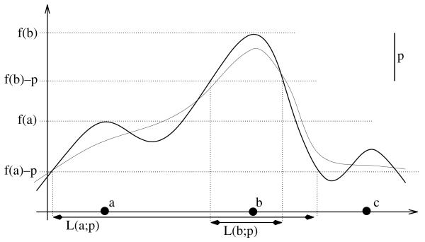
The graph of a 1D function f is shown as the thick solid curve. The magnitude of the persistence threshold p is the length of the interval in the upper right. Notice that f assumes the largest value in L(b;p) at b. This means that b is a persistent maximum of f. The other two local maxima are not persistent, for example the largest value of f in L(a;p) is assumed at b, not at a. The thin curve shows a perturbation of f that is within p/2 away from f and has only one maximum close to b (more precisely, in L(b;p)).
Because of noise, persistent maxima can occur essentially anywhere inside constant high intensity regions. In order to make them closer to the centerlines of small vessels, we apply a 3D low pass filter to the data before computing the persistent maxima. For all examples discussed in this paper, eight iterations of the 2 × 2 × 2 box filter were used for this purpose.
Persistence of all maxima in a 2D slice can be computed in O(nlogn) time (where n is the number of pixels in the slice) using the procedure of Edelsbrunner et al., 2001. First, we initialize a variable Pu for each pixel u to zero. After the algorithm terminates, the value of Pu for any pixel u which is a local maximum will be equal to its persistence. For pixels u which are not local maxima, Pu will be zero. Starting from S = Ø, we keep inserting pixels of the slice in order of decreasing intensity into S. As we do that, we keep track of the connected components (determined based on 8-neighborhoods) of the union of pixels inserted so far using the union-find datastructure (Cormen et al., 1990, Chapter 21). For each connected component, we keep track of the maximum intensity pixel within that component. Whenever a new pixel w of intensity I is inserted, the union-find data structure as well as the location of the maximum are updated. All connected components of the neighbors of w of intensity greater than I are merged to one. Its highest intensity pixel is computed as the brightest pixel among the merged components’ maximum intensity pixels. For each of the merged connected components, if v is its maximum intensity pixel and Iv is its intensity, we update Pv to Iv − I. The procedure terminates after all pixels are inserted into S.
The 2D procedure described above allows one to compute a volume dataset that can be used to efficiently generate the set of persistent maxima for any persistence threshold as follows. We run the 2D algorithm for every slice perpendicular to one of the coordinate axes, recording the results in a 3D array of the same dimensions as the input 3D image. This yields three arrays, one per coordinate axis. We take entry-wise maximum of these arrays, obtaining a 3D array that we call persistence volume. For a threshold M, the set A of persistent maxima on 2D slices that we use as a starting point for the blood vessel reconstruction consists of centers of voxels of the persistence volume that have value larger than M.
Because of large sizes of the CT scans, computing persistent maxima is the most computationally intensive phase of our algorithm (for all test datasets described in Section 5, at least 95% of time is spent on computing the persistent maxima). The forest operations described in Section 4 act on the set of persistent maxima, which is relatively small; therefore, in practice, they run much faster. Saving the persistence volume and using it to generate the persistent maxima facilitates experimenting with different persistence thresholds. At the same time, it carries negligible overhead over the best method for compute all persistent local maxima on 3D axis-oriented slices for a prescribed threshold we are aware of (which is based on the same idea).
4. Vessel reconstruction from the persistent maxima
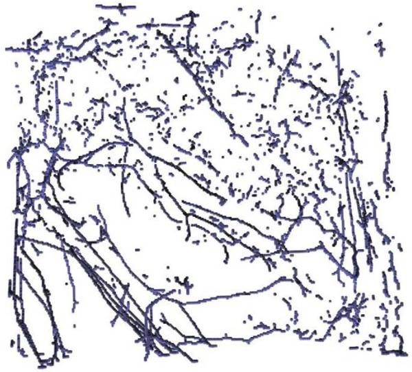
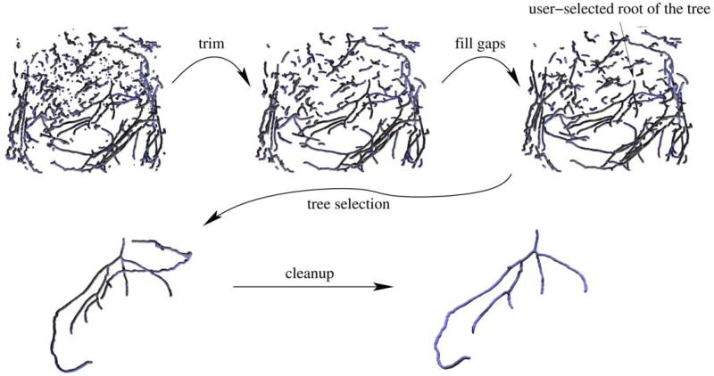
Points of the set A of persistent maxima tend to be concentrated along the centerlines of blood vessels. There are numerous outliers that do not belong to any vessel, but their distribution tends to be structureless. The procedure described in this section attempts to connect the neighboring points on the same blood vessel trees. We first compute a forest (i.e., a graph with no loops) F connecting the points in A with short edges, which serves as a crude reconstruction of the blood vessels. This forest is subsequently cleaned up and improved using simple geometric filters (Fig. 4). First, short branches are trimmed. Then, ‘gaps’ in the vessels are filled by finding branches that seem to geometrically fit to each other and connecting them with edges. The user interactively selects the root of the tree of interest (i.e., the point from which blood flows into the tree). Finally, the user-selected tree is cleaned up by removing branches that either lead to sharp turns in the blood flow direction predicted from our reconstruction or are well-aligned with blood vessels outside the tree of interest. Below we describe each step in more detail.
4.1. Building the forest
The purpose of this step is to build a forest F, serving as a crude reconstruction of the vessels in the image, from the 3D point set A. Since the points in A tend to be densely distributed along the vessels, it is natural to build F by connecting nearby points in A. More precisely, we construct F as the minimum forest that uses edges connecting the points in A shorter than a certain threshold using the Kruskal’s minimum spanning tree algorithm (Cormen et al., 1990, Chapter 23). We sort the edges connecting the points of A whose length is smaller than the threshold according to length. To generate all edges shorter than the threshold efficiently, we arrange the points in the octree datastructure (described in, for example, Samet, 1990). Then, we attempt to insert the edges into the forest one at a time in order of increasing length. As we do that, we keep track of the connected components of the forest using the union-find data structure (Cormen et al., 1990, Chapter 21). Edges whose endpoints belong to the same connected component are not inserted into the tree (since this would cause a loop in the graph).
Let us note that the idea of using Euclidean minimum spanning tree for geometric reconstruction from points is not new. The work in de Figueiredo and Gomes (1995) contains an in-depth analysis of this approach to curve reconstruction in the planar case.
4.2. Forest trimming
Some points in A can be somewhat off the axis of the blood vessels or are outliers defined by intensity maxima at random places. This typically leads to numerous short branches of the trees in F. Similar problems arise when computing skeletons of shapes, where noise and sharp features can lead to numerous branches which can be pruned to make the skeleton easier to comprehend (Ogniewicz and Kübler, 1995). The purpose of forest trimming is to remove such short branches. We do that by iteratively removing the shortest branch in the forest until the length of all branches is above a certain threshold.
For the purpose of this procedure, we treat leaf vertices of the forest F as branch endpoints. The branch of a leaf vertex v is defined as the simple path (i.e., path that uses no vertex more than once) in the forest starting at v and ending at a vertex of degree other than 2. In order to efficiently keep track of short branches due to be removed we use a priority queue. At startup, all leaf nodes of the forest are inserted into the queue. The cost of a leaf node is equal to the length of its branch.
The main loop takes a least cost leaf vertex off the queue and removes all edges in its branch. Such a removal may potentially change the length of some leaf vertices’ branches. This happens whenever the last vertex w of the branch has degree 2 after the removal. In such cases, we trace the two paths starting at w until they reach a vertex of degree other than 2. Let the endpoints of these paths be w1 and w2 and their lengths be l1 and l2. If the degree of w1 or w2 is one, its cost should be updated to l1 + l2. This is illustrated in Fig. 5. We implement this by simply inserting the endpoints with new priorities into the queue. This means an endpoint can appear in the queue more than once, and that some of these instances may have outdated priorities. However, the priorities of branches can only decrease in time (as their length can only increase) and therefore we can detect whether a leaf taken off the queue is valid or not by checking how many times it appears on the queue: if it appears just once before it is taken off, it means that its cost is valid. In order to be able to do that efficiently, for each vertex we maintain the number of times it appears on the queue.

An example showing that a branch length (and therefore also the cost) can change after a removing a branch from the forest. The shortest branch of the tree on the left (dotted line in the figure on the right) is removed. The length of the branch shown as the thick line increases by the length of the path shown as the dashed line.
The procedure terminates when the length of the branch taken off the queue is above the threshold.
4.3. Gap filling
In some cases, the points in A are not dense enough along a blood vessel for the tree growing algorithm to obtain its continuous reconstruction. This is typically caused by variation of contrast along the blood vessels: in the low contrast parts the persistence of the local maxima on 2D slices drops below the threshold and, consequently, they are not included in A. We attempt to fix this problem by adding edges connecting leaf vertices in the forest that appear to belong to the same blood vessel based on the following principles:
Since gaps tend to be small, u and v should not be too far from each other.
The newly inserted edge should blend well with the tree branches starting at u and v. This means that the outward-pointing tangent vector to the vessel at u should point in a direction close to the vector
This naturally leads to the following penalty function defined for all pairs of leaf vertices:
where | · | denotes the Euclidean norm of a vector, Tu and Tv are outward pointing tangent vectors at u and v and α is a scaling constant, determined experimentally. To estimate the tangent vector Tu at u, we follow the path in the graph starting from u. The path is terminated as it reaches a prescribed length or it hits a junction (vertex of degree greater than 2), whichever happens first. We approximate Tu as the vector from the endpoint of the path to u. The tangent at v, Tv, is estimated in the same way.
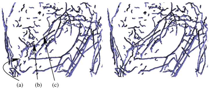
Our algorithm greedily connects pairs of leaf vertices in order of increasing penalty, stopping when the penalty exceeds a certain threshold. We reject edges that would cause loops to appear in the graph. This can be implemented efficiently by utilizing the union-find data structure in the same way as in the Kruskal’s minimum spanning tree algorithm. Fig. 6 shows the result of the gap filling stage for one of the test datasets.
4.4. Tree selection
So far we were operating on the entire forest, that typically includes all blood vessel trees reconstructed by our algorithm. Now, the user needs to select a blood vessel tree of interest from this forest. The selection is made by clicking on a voxel near the root of the tree of interest. We find its nearest node in the forest and output its connected component. The connected component is computed using the depth-first search algorithm (Cormen et al., 1990, Exercise 22.3-11). As illustrated in Figs 4, ,77 and and8,8, this tree may potentially contain spurious branches that need to be cleaned up. Note that the root node selected by the user should define the point from which the blood flows into the tree in order for the tree cleanup step (described next) to work properly.
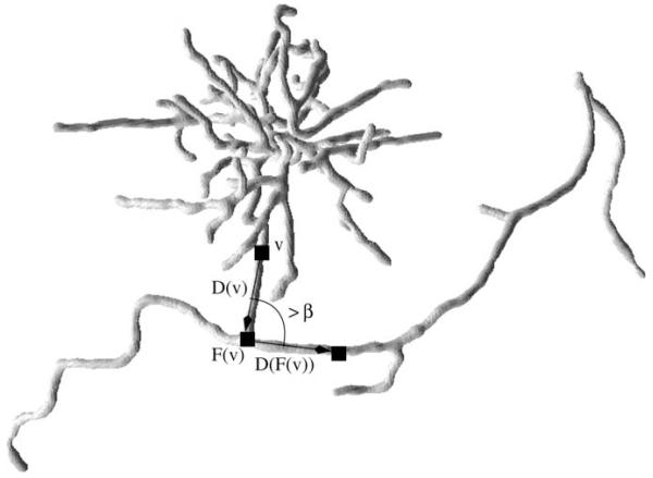
An example of a sharp turn in a tree arising from one of the datasets. The branch ending in a complex configuration (in fact, artifact arising from a pacemaker lead, slices of the same dataset are shown in Fig. 11) does not belong to the coronary tree and is removed based on the sharp turn heuristic (because the angle between the vectors D(v) and D(F(v)) shown in the figure exceeds the threshold).
4.5. Tree cleanup
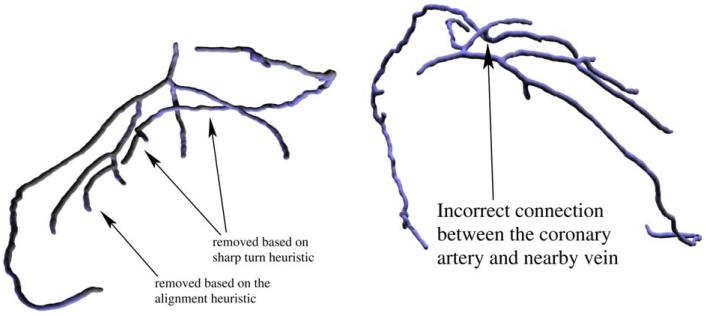
We use two simple geometric heuristics to detect and remove spurious branches from the user-selected tree. An example where both heuristics are necessary is shown in Fig. 8.
4.5.1. Sharp turns in the blood flow direction
We first direct the edges of the tree so that they point toward the root (i.e., so that by following the directed edges from any vertex one can obtain a simple path leading to the root). The directions can be thought as opposite to the blood flow direction (assuming blood flows out of the root into the tree) and hence should not abruptly change. Building upon this observation, we detect and remove edges that lead into sharp turns. The details are described below.
For each vertex v of the directed tree, we follow its path toward the root until it gets longer than some minimum length L or it reaches the root. Let the endpoint of this path be F(v). Denote the vector from v to F(v) by D(v). This is our estimate of the direction opposite to the blood flow. We first mark all vertices v of the tree for which the angle between D(v) and D(F(v)) is greater than a certain threshold β. Then, for each marked vertex we trace its path in the tree until its length exceeds L or it reaches a vertex of degree other than 2 (whichever happens first) and remove its last edge. Finally, we compute the connected component of the resulting forest that contains the root vertex. An example of branches removed based on the sharp turn criterion are shown in Figs. 7 and and88.
4.5.2. Alignment with branches representing other blood vessels
Some branches belonging to other vessels are not detected using the procedure described previously. An example is shown in Fig. 8. There is a vein running very close to several branches of the coronary tree. Parts of the vein form spurious branches of the tree. The biggest branches can be removed based on the sharp turn heuristic described previously. However, the smallest branch does not form a sharp angle with the coronary artery. Still, Fig. 8 contains a clear indication that the branch does not belong to the tree: it is aligned well with another branch (in this case, one of the branches removed based on the sharp turn heuristic) which appears to be its continuation. This observation naturally leads to the following procedure.
Let T be the tree to be cleaned up and F the forest resulting from the forest trimming operation described in Section 4.2. Consider a simple path P in T starting at a vertex v of degree greater than 2 and terminating at a vertex of degree other than 2. We can estimate the outward tangent vector Tv for P at v as in Section 4.3:
If the alignment measure is less than a certain prescribed threshold a for some vertex u as described above, we remove the first edge of the path P from T.
After examining all paths P described above we compute the connected component of the resulting forest (i.e., T with certain edges removed) containing the root. This is the final reconstruction of the vascular tree.
5. Results
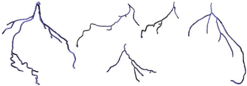
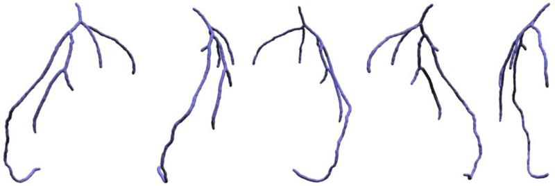
Our algorithm has been run on five different datasets (heart CT scans). The resulting coronary trees are shown in Fig. 9. Different views of the same tree are shown in Fig. 10. Generally, the algorithm was able to correctly capture the structure of the coronary arteries, even for a dataset with artifacts caused by a pacemaker lead (Fig. 11). The outcome obviously depends on the choice of the algorithm’s parameters and thresholds. An example of a dataset for which selecting parameters turned out to be difficult is shown in Fig. 12. The tree generated from that dataset contains two short spurious branches. One branch is not followed correctly because of low contrast over a few consecutive slices (even though contrast improves and the branch is clearly visible over the subsequent 100 slices) and one is completely missed. Still, the major branches of the coronary tree were reconstructed correctly. We also expect that in certain cases (for some datasets or for suboptimal choices of the parameters) the tree generated by our algorithm may include parts of nearby veins (cf. Fig. 8).
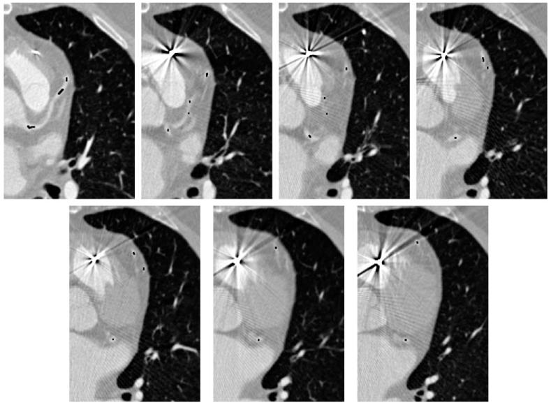
Slices of a dataset with artifacts caused by a pacemaker lead. Despite the poor quality of data, our procedure is able to track the coronary artery correctly (the black dots were obtained by scan-converting the output tree).
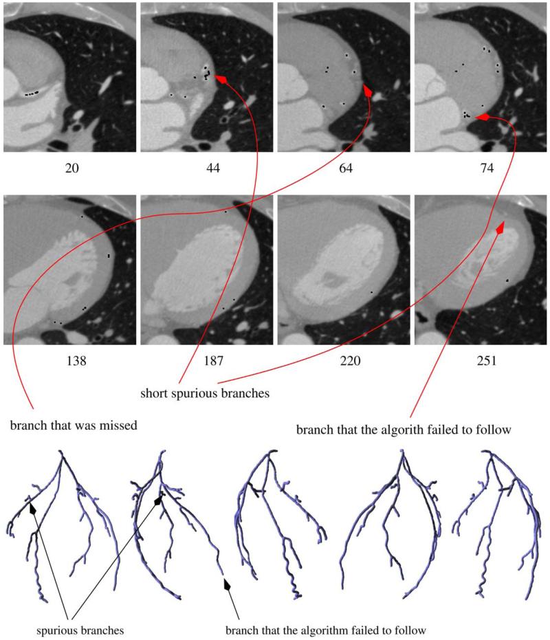
Top: slices of a dataset showing potential problems of our approach (black dots are obtained by scan-converting the reconstructed tree). The algorithm fails to follow one of the branches because of low contrast over a number of slices (the branch is hardly visible in slice 220; even though it becomes clearly visible again a few slices later and A contains points generated from the 228th and most of the subsequent slices, gap filling fails because of wiggly shape of the artery in this area), generates a two short spurious branches (two of which can be seen on the slices presented above) and misses one branch (weak near the bifurcation) completely. Bottom: the reconstructed coronary tree rendered from five different viewpoints.
Prior to being used as the input to our procedure, we equalized the mean and standard deviation of the intensity on the slices of the input dataset. This is important because of substantial differences in the statistics of the intensities on (even close) different slices. We also applied a low pass filter (in this case, 8 iterations of the 2 × 2 × 2 box filter; cf. discussion in Section 3). The image leading to the leftmost tree in Fig. 9 has been acquired using a Siemens Sensation 64 CT scanner (Forcheim, Germany) with a spatial resolution of 0.4 × 0.4 × 0.6 mm. The images leading to the other four trees were obtained using a Siemens Sensation 16 scanner with 0.6 × 0.6 × 1.0 mm resolution. In all cases, retrospectively ECG-gated spiral acquisition was used and 70 cc of Ultravist 370 (Schering, Germany) contrast followed by 30 cc of saline flush at a rate of 5 cc/s was administered to the patients.
The datasets were cropped before running our algorithm to reduce their size to between 10 and 15 million voxels. The running times of our implementation (currently far from optimal) were about 6 min for each of the datasets on a Pentium III-850 MHz workstation. Most of this time was spent on computing the persistence volume described in Section 3. The rest of the procedure took less than 15 s for every tree shown in Fig. 9.
5.1. User-defined parameters
Our algorithm requires fixing several parameters: the persistence threshold M for local maxima, the maximum edge length L for use in the forest growing phase, minimum length of a branch m to be used when trimming, the α parameter and the maximum allowable penalty function value S for gap filling purposes, angle and alignment and distance thresholds β, a and K for the cleanup stage. We found out that, although the number of these parameters is high, they are relatively easy to set and, once they are set, they tend to work well for all datasets coming from the same source. In particular, all trees shown in Fig. 9 except for the one on the left were extracted from four different datasets acquired using the same CT scanning device. For all of them, we used the same parameters, determined after about half an hour of experiments on one of the datasets: M equal to about 5% of the maximum intensity, L = 7, m = 10, α = 0.02, S = 1, β = 85°, a = 1 and K = 10 (assuming the grid is of size 1 in x and y dimensions). When computing vectors tangent to branches or paths on the gap filling or cleanup stages, we trace paths in the forest until they reach length 10 (or to the closest junction). Recall that our algorithm spends most of the time computing the persistence volume, which can be reused for different thresholds. Consequently, the user can see the result of his/her parameter adjustments in less than 15 s once the persistence volume is computed.
Perturbing the parameters induces easily predictable changes to the output tree. For example, lower maximum penalty for gap filling might make some branches shorter. Higher β or lower a might cause some of the spurious branches to survive.
6. Discussion and future work
We presented a simple and effective algorithm allowing one to extract coronary trees from heart CT scans. We hope that the trees extracted using our procedure could be used as initial conditions for active contour models, speeding up their convergence and improving the segmentation results. They could also help supplement active contours with constraints that could help prevent leaks or instability. We believe that, apart from extracting blood vessel trees of various types, variations of our procedure could be applicable to other problems where reconstruction of tree-like (or, more generally, graph-like) structures is of importance: extracting neuron cells and their connections from confocal microscopy data, airways from 3D lung images etc.
There are several technical improvements of the algorithm that we are planning to pursue in the future. The persistent maxima computation procedure could be augmented with additional criteria allowing one to reject some of the persistent maxima. For example, one could extract a superset of the heart from the image (e.g., by applying a low pass filter of a small cutoff frequency and thresholding the resulting image) and then use it to conservatively reject the maxima outside the heart. In addition, the vesselness measure of Frangi et al. (1998) can be used to eliminate even more maxima. Although this approach is very effective in preserving points on the coronary arteries and rejecting outliers (Fig. 13), it turns out to have little effect on the final outcome of the algorithm: the reconstructed vessel trees were essentially the same as in Fig. 9. Nevertheless, we expect that this and other heuristics allowing one to improve the point set the forest is reconstructed from might prove useful in future.

Comparison of forests constructed from the candidate points (before applying the forest filters): left, persistent maxima (computed as described in Section 3); center, persistent maxima with those conservatively decided to lie outside the heart removed; right, additionally, 70% of points of smallest vesselness measure were removed.
The trees extracted by the algorithm as described in this paper typically pass through the calcified plaque areas if they exist, because of their high intensity. The plaque can be detected by examining the variation of intensity along the tree. More generally, one could perform more detailed intensity analysis in the vicinity of the coronary tree to estimate the artery width, find soft plaque, aneurysms, stenoses or other abnormalities of interest. Such analysis might also lead to improvements of the reconstructed coronary tree, for example by providing methods to detect spurious branches shown in Fig. 12.
Finally, we are interested in a more precise validation of our results and detailed comparison to competing methods such as those described in Section 2. This could be done by using phantom models of vessel trees as in Dietrich et al. (2002) or precise labelling of vessel branches or bifurcations in the automatically reconstructed trees and comparing them with those present in manual segmentations provided by several human experts as in Bullitt et al. (2001). Yet another approach could be to use images of animal hearts and compare them with dissection results.
Acknowledgements
This work is part of the National Alliance for Medical Image Computing (NAMIC), funded by the National Institutes of Health through the NIH Roadmap for Medical Research, Grant U54 EB005149. This work was also supported by a Grant from NIH (NAC P41 RR-13218) through Brigham and Women’s Hospital and NSF Grants DMS-0138420 and DMS-0107396.
References
- Aylward S, Bullitt E. Initialization, noise, singularities, and scale in height ridge traversal for tubular object centerline extraction. IEEE Transactions on Medical Imaging. 2002;21(2):61–75. [Abstract] [Google Scholar]
- Aylward S, Bullitt E, Pizer S, Eberly D. Intensity ridge and widths for tubular object segmentation and description; Proceedings of IEEE/SIAM Workshop Mathematical Methods Biomedical Image Analysis; 1996.pp. 131–138. [Google Scholar]
- Bühler K, Felkel P, La Cruz A. Geometric methods for vessel visualization and quantification – a survey, Technical Report TR_VRVis_2002_035. VRVis Research Center; Vienna, Austria: 2002. [Google Scholar]
- Bullitt E, Aylward S, Smith K, Mukherji S, Jiroutek M, Muller K. Symbolic description of intracerebral vessels segmented from MRA and evaluation by comparison with X-ray angiograms. Medical Image Analysis. 2001;5:157–167. [Abstract] [Google Scholar]
- Bulpitt AJ, Berry E. Spiral ct of abdominal aneurysms: comparison of segmentation with an automatic 3-d deformable model and interactive segmentation. Proceedings of SPIE. 1998;3338:938–946. [Google Scholar]
- Chung ACS, Noble JA, Summers P. Fusing speed and phase information for vascular segmentation of phase contrast MR angiograms. Medical Image Analysis. 2002;6:109–128. [Abstract] [Google Scholar]
- Chung ACS, Noble JA, Summers P. Vascular segmentation of phase contrast magnetic resonance angiograms based on statistical mixture modeling and local phase coherence. IEEE Transactions on Medical Imaging. 2004;23(12):1490–1507. [Abstract] [Google Scholar]
- Cormen T, Leiserson C, Rivest R. Introduction to Algorithms. McGraw-Hill; New york: 1990. [Google Scholar]
- de Figueiredo LH, Gomes J. Computational morphology of curves. The Visual Computer. 1995;11(2):105–112. [Google Scholar]
- Deschamps T, Cohen LD. Grouping connected components using minimal path techniques. Application to reconstruction of vessels in 2D and 3D images. Proceedings of the Computer Vision and Pattern Recognition (CVPR) 2001;2:102–109. [Google Scholar]
- Deschamps T, Cohen LD. Fast extraction of tubular and tree 3D surfaces with front propagation methods; Sixteenth International Conference on Pattern Recognition, ICPR 2002; 2002.pp. 731–734. [Google Scholar]
- Dietrich O, Nikolaou K, Wintersperger BJ, Flatz W, Nittka M, Petsch R, Kiefer B, Schoenberg SO. iPAT: applications for fast and cardiovascular MR imaging. Electromedica. 2002;70:133–145. [Google Scholar]
- Edelsbrunner H, Harer H, Zomorodian A. Symposium on Computational Geometry, ACM. ACM Press; New York, NY, USA: 2001. Hierarchical morse-smale complexes for piecewise linear 2-manifolds; pp. 70–79. [Google Scholar]
- Felkel P, Wegenkittl R, Kanitsar A. Vessel tracking in peripheral CTA datasets – an overview; Proceedings of the Seventeenth Spring conference on Computer graphics, IEEE Computer Society, SCCG 2001; Washington, DC, USA. 2001.p. 232. [Google Scholar]
- Florin C, Moreau-Gobard R, Williams J. Automatic heart peripheral vessels segmentation based on a normal MIP ray casting technique; Proceedings MICCAI 2004; Saint-Malo, France. 2004. pp. 483–490. [Google Scholar]
- Frangi A, Niessen W, Vincken K, Viergever M. Proceedings of Medical Image Computing and Computer-Assisted Intervention, MIC – CAI 1998. 1998. Multiscale vessel enhancement filtering; pp. 130–137. [Google Scholar]
- Frangi AF, Niessen WJ, Hoogeveen RM, van Walsum T, Viergever MA. Model-based quantitation of 3-d magnetic resonance angiographic images. IEEE Transactions on Medical Imaging. 1999;18:946–956. [Abstract] [Google Scholar]
- Kanitsar A, Fleischmann D, Wegenkittl R, Sandner D, Felkel P, Gröller E. Computed tomography angiography: a case study of peripheral vessel investigation; VIS 2001, Proceedings of the conference on Visualization 2001. IEEE Computer Society; Washington, DC, USA. 2001.pp. 477–480. [Google Scholar]
- Kass M, Witkin A, Terzopoulos D. Snakes: active contour models. International Journal of Computer Vision. 1988;1:321–331. [Google Scholar]
- Kirbas C, Quek F. A review of vessel extraction techniques and algorithms. ACM Computing Surveys. 2004;36(2):81–121. [Google Scholar]
- Krissian K, Malandain G, Ayache N, Vaillant R, Trousset Y. Model-based multiscale detection of 3D vessels; Proceedings of the IEEE Conference on Computer Vision and Pattern Recognition, CVPR; Santa Barbara. 1998.1998. pp. 722–727. [Google Scholar]
- Lorigo L, Faugeras O, Grimson W, Keriven R, Kikinis R, Nabavi A, Westin C-F. Codimension-two geodesic active contours; Proceedings of CVPR.2000. pp. 1444–1451. [Google Scholar]
- McInerney T, Terzopoulos D. Deformable models in medical images analysis: a survey. Medical Image Analysis. 1996;1(2):91–108. [Abstract] [Google Scholar]
- McInerney T, Terzopoulos D. Topology adaptive deformable surfaces for medical image analysis. IEEE Transactions on Medical Imaging. 1999;18:840–850. [Abstract] [Google Scholar]
- Nain D, Yezzi A, Turk G. Vessel segmentation using a shape driven flow; Proceedings of MICCAI; St. Malo, France. 2004.pp. 51–59. [Google Scholar]
- National Center for Health Statistics, Health, United States . With Chartbook on Trends in the Health of Americans. Hyatsville, Maryland: 2004. Available from: < http://www.cdc.gov/nchs/hus.htm>. [Abstract] [Google Scholar]
- Ogniewicz RL, Kübler O. Hierarchic voronoi skeletons. Pattern Recognition. 1995;28(3):343–359. [Google Scholar]
- Pizer SM, Eberly D, Fritsch DS, Morse BS. Zoom-invariant vision of figural shape: the mathematics of cores. Computer Vision and Image Understanding. 1998;69(1):55–71. [Google Scholar]
- Samet H. Applications of Spatial Data Structures. Addison-Wesley; Reading, MA: 1990. [Google Scholar]
- Sethian JA. Level Set Methods and Fast Marching Methods: Evolving Interfaces in Computational Geometry, Fluid Mechanics, Computer Vision and Materials Science. Cambridge University Press; Cambridge: 1999. [Google Scholar]
- Wesarg S, Firle EA. Segmentation of vessels: the corkscrew algorithm. In: Proceedings of SPIE Medical Imaging 2004. 2004;3:1609–1620. [Google Scholar]
- Wink O, Niessen WJ, Viergever MA. Fast delineation and visualization of vessels in 3-D angiographic images. IEEE Transactions on Medical Imaging. 2000;19(4):337–346. [Abstract] [Google Scholar]
- Yim PJ, Choyke PL, Summers RM. Gray-scale skeletonization of small vessels in magnetic resonance angiography. IEEE Transactions on Medical Imaging. 2000;19(6):568–576. [Abstract] [Google Scholar]
- Yim PJ, Cebral JJ, Mullick R, Marcos HB, Choyke PL. Vessel surface reconstruction with a tubular deformable model. IEEE Transactions on Medical Imaging. 2001;20(12):1411–1421. [Abstract] [Google Scholar]
Full text links
Read article at publisher's site: https://doi.org/10.1016/j.media.2006.05.002
Read article for free, from open access legal sources, via Unpaywall:
https://europepmc.org/articles/pmc3640425?pdf=render
Citations & impact
Impact metrics
Citations of article over time
Alternative metrics
Smart citations by scite.ai
Explore citation contexts and check if this article has been
supported or disputed.
https://scite.ai/reports/10.1016/j.media.2006.05.002
Article citations
Automatic Coronary Artery Segmentation Using Active Search for Branches and Seemingly Disconnected Vessel Segments from Coronary CT Angiography.
PLoS One, 11(8):e0156837, 18 Aug 2016
Cited by: 9 articles | PMID: 27536939 | PMCID: PMC4990346
Automated generation of directed graphs from vascular segmentations.
J Biomed Inform, 56:395-405, 09 Jul 2015
Cited by: 4 articles | PMID: 26165778 | PMCID: PMC4547695
Digital Topology and Geometry in Medical Imaging: A Survey.
IEEE Trans Med Imaging, 34(9):1940-1964, 14 Apr 2015
Cited by: 20 articles | PMID: 25879908
Review
Unraveling flow patterns through nonlinear manifold learning.
PLoS One, 9(3):e91131, 10 Mar 2014
Cited by: 4 articles | PMID: 24614890 | PMCID: PMC3948738
Automatic centerline extraction of coronary arteries in coronary computed tomographic angiography.
Int J Cardiovasc Imaging, 28(4):921-933, 03 Jun 2011
Cited by: 39 articles | PMID: 21637981 | PMCID: PMC3360862
Go to all (10) article citations
Similar Articles
To arrive at the top five similar articles we use a word-weighted algorithm to compare words from the Title and Abstract of each citation.
Validation of image-based method for extraction of coronary morphometry.
Ann Biomed Eng, 36(3):356-368, 29 Jan 2008
Cited by: 25 articles | PMID: 18228141
A novel 3D multi-scale lineness filter for vessel detection.
Med Image Comput Comput Assist Interv, 10(pt 2):436-443, 01 Jan 2007
Cited by: 2 articles | PMID: 18044598
Robust feature classification and editing.
IEEE Trans Vis Comput Graph, 13(1):34-45, 01 Jan 2007
Cited by: 4 articles | PMID: 17093334
A review of 3D/2D registration methods for image-guided interventions.
Med Image Anal, 16(3):642-661, 13 Apr 2010
Cited by: 215 articles | PMID: 20452269
Review
Funding
Funders who supported this work.
NCRR NIH HHS (2)
Grant ID: P41 RR 13218
Grant ID: P41 RR013218
NIBIB NIH HHS (2)
Grant ID: U54 EB005149
Grant ID: U54 EB 005149
