Abstract
Free full text

Partial Isotope Profiles are Sufficient for Protein Turnover Analysis using Closed-form Equations of Mass Isotopomer Dynamics
Abstract
Metabolic labeling with atom-based heavy isotopes, followed by LC-MS, has been a powerful technique for studies of proteome and metabolome. In proteomics, protein turnover of thousands of proteins can be estimated from the gradual incorporation of 2H or 15N in the diet. Software tools have been developed to automate the estimation of protein turnover. Traditionally, the turnover has been estimated using the time-course of the depletion of the normalized abundance of monoisotope. While the bioinformatics aspects of peak detection and integration, time-course modeling, and uncertainty estimation have progressed, mass isotopomer dynamics during label incorporation has only been modeled from approximate approaches or numerical simulations.
We derive closed-form equations that describe the dynamics of mass isotopomers during metabolic labeling with an atom-based stable isotope. The derived equations create an alternative method for estimating label incorporation. They also provide opportunities for estimations of precursor-product relationships in species or systems where they are unknown. The equations are useful in bioinformatics tools for analyzing mass spectral data from metabolic labeling.
Introduction
Metabolic labeling with stable isotopes followed by liquid-chromatography coupled into mass spectrometry (LC-MS) has been used to study the turnover of proteins, lipids, and other biomolecules in vivo1. For protein turnover studies, labeled samples are processed via standard proteomics workflows2. The labeling is quantified via changes in the isotope profiles of peptides. In a widely-used approach, the time-course of the relative abundance (normalized by the sum of all mass isotopomers) of the monoisotope is used in an exponential decay model to extract the degradation rate constant (DRC) of a protein3.
Atom-based labeling4 (such as labeling with 2H or 15N) often creates overlapping isotope profiles of labeled and unlabeled peptides. For example, labeling with heavy water (2H labeling) is partial, since less than 10% enriched water is provided to model organisms (high doses of heavy water are toxic). The isotope profiles of labeled species are simulated using a model where the labeling atom is designated as a new atom “type” with a different isotope pattern5. For example, in heavy water labeling, hydrogens, which are accessible to the deuterium in heavy water, are designated as belonging to an atom “type” with the 2H isotope abundance of (pH + pX), and 1H isotope abundance of (1 - pH - pX). Here, pH is the relative abundance (RA) of 2H in nature; pX is the RA of 2H incorporated from the heavy water into the biomolecule. Numerical techniques6–8 (for example, Fast-Fourier transforms, or multinomial distribution) are used to calculate the isotope profiles of labeled species at various values of pX. The calculations are used to determine pX from the fit of the theoretical profiles into the experimental observation5, or for the estimation of the number of 2H atoms incorporated into the biomolecule at the enrichment plateau9. In this work, we show that closed-form equations govern the dynamics of the abundances of the mass isotopomers during labeling.
The abundances of mass isotopomers of a labeled species are time-dependent during the labeling. However, for heavy mass isotopomers, only the isotopologues that originate from the labeling atom “type” change during the labeling. The rest of the heavy isotopologues are time-invariant. Therefore, we separate the isotopologues of the labeling atom “type” from those of the rest of the atoms in a biomolecule. The modeling of the mass isotopologues of the labeling atom “type” leads to closed-form equations linking the abundances (both raw and normalized) of mass isotopomers during metabolic labeling. The equations can be used in alternative approaches to analyzing mass spectral data from metabolic labeling. As an example, we show how to calculate rate constants using raw abundances of two mass isotopomers. The derivations are presented for deuterium enrichment of peptides resulting from heavy water labeling. However, the equations are general. They can be used for other atom-based labeling agents4, 10–11, such as 15N and 12C, or for other biomolecules such as lipids12.
2.1. Data Description.
We used a large-scale data set of the liver proteome of (low-density lipoprotein receptor knock-out) LDLR−/− mice fed a normal diet13. The data set consists of 127 LC-MS experiments. They were performed in six times points of label duration. Peptide samples were prepared from eleven SDS-PAGE bands. Each sample was run in duplicate. Mass spectral data were collected using Q Exactive™ Plus Hybrid Quadrupole-Orbitrap™ Mass Spectrometer (Thermo Scientific, CA). Mascot14 database search engine was used for peptide identification. It calculates the global false discovery rate (we set it at 5%) by using matches to the reversed sequences. The data set is available at ProteomeXChange site (PXD009493). It contains 21706 unique peptides, which have been quantified in at least four out of the six labeling timepoints. The R scripts written for numerical simulations in this work are available at http://dynamic-proteome.utmb.edu/MIDynamics/MIDynamics.aspx.
2.2. Novel closed-form equations of mass isotopomer dynamics during metabolic labeling
We will use three forms of a reference to mass isotopomers of a peptide. Mk refers to the kth mass isotopomer (k = 0 is the monoisotope). It will not designate any abundance. Ik(t) applies to the RA of the kth mass isotopomer at the labeling time t. Ak(t) applies to the MS measured raw (non-normalized) abundance of the kth mass isotopomer. Mass isotopomers result from the combination of the isotopologues with the same nominal mass. The time-course of I0(t) is used to determine the protein degradation rate constant, k, via an exponential decay model3:
where I0asymp is the asymptotic (after reaching the plateau of labeling) RA of the monoisotope.
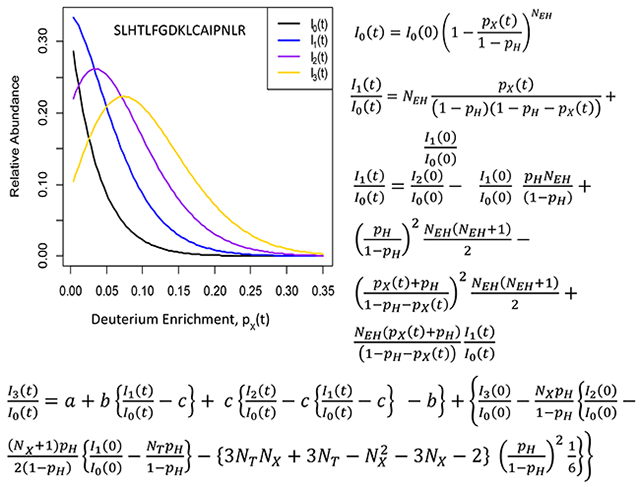
The isotope distribution of a peptide in metabolic labeling with water is modeled by separating peptides’ hydrogen atoms into two groups5, 15. In the first group are the hydrogens that are non-accessible to the deuterium. In the second group are the hydrogens that can be labeled by the deuterium in heavy water. The number of hydrogens in the second group we denote as NEH. We refer to this hydrogen type as XH. The relevant probabilities of 2H for each group are pH and (pH + pX(t)), respectively. Here, pH is the natural abundance of deuterium, and pX(t) is the deuterium enrichment in a peptide from the heavy water at the labeling duration time t. Details of the derivations of the following closed-form equations are provided in Supporting Information. Here, we note that the time-dependent isotopologues originate from the deuteriums of XH. The equation for the time-course evolution of I0(t) is:
pX(t) is also referred to as molar percent excess (MPE). When the labeling of a protein reaches its plateau, (pX(t)+pH) is equal to pW (2H enrichment of heavy water). An important feature of Eq. (2) is that it depends on the normalization at two different timepoints of labeling; 0 and t. Therefore, only RAs can be used in this equation.
By separating the probability of the isotopologue originating from the labeling of XH from the other isotopologues of M1, one obtains the following equation for I1(t):
The first term in the sum originates from the M1 isotopologue of XH. The second term is the sum of all M1 isotopologues, except the isotopologue of XH. By substituting Eq. (2) into Eq. (3), we obtain the following relationship for the time-course of the I1(t)/I0(t) ratio:
Previously, Anderson and coworkers16 have discussed that the I1(t)/I0(t) ratio can be expanded as a sum of probabilities of the isotopologues of M1. Eq. (4) presents the explicit form of the time dependency of the I1(t)/I0(t) ratio on the label enrichment, pX(t), of a peptide. An important aspect of Eq. (4) is that it can use non-normalized abundances of the monoisotope and the first heavy mass isotopomer as measured in LC-MS. From Eq. (4), we determine the deuterium enrichment, pX(t), of a peptide:
Eq. (5) is important because, on the right-hand side, there is a dependency on the A1(t)/A0(t) ratio and
Starting from the probabilities of all isotopologues of M2, we have derived the following closed-form equation for the time-course evolution of the ratio of raw abundances of M2 and M0:
The derivations of Eqs. (3) and (6) are provided in Supporting Information. Eq. (6) links three raw abundances, A0(t), A1(t), and A2(t), with the deuterium enrichment of a peptide, pX(t), and its number of exchangeable hydrogens, NEH. Eq. (6) is exact; no approximations have been made in its derivation. The correctness of the equation can be seen from the asymptotic behaviors and will numerically be validated below.
Eq. (5) relates NEH and pX(t) via the time-course of the A1(t)/A0(t) ratio. We recast the equation to the form shown below to emphasize the calculations of NEH:
Eqs. (4) and (6) constitute a system of two equations for two variables - NEH and pX(t). Theoretically, they should determine the variables exactly at every time point of labeling from raw abundances of the first three mass isotopomers. Hellerstein and coworkers9 have determined NEH values from the mass isotopomer distributions of peptides at the plateau enrichment of a protein. Their approach9 generated mass isotopomer distributions from combinatorial simulations with different NEH values to determine the optimal value. At the plateau of label incorporation, (pX(t)+pH) in Eq. (7) is equal to pW. Given body water enrichment with deuterium, pW, Eq. (7) determines NEH values without simulations and using only the raw abundances of the first two mass isotopomers.
We have also derived the time evolution equation for the third heavy mass isotopomer, M3:
In Eq. (8), NT is the number of all hydrogen atoms in a molecule, a(t), b(t), and c(t) are time-dependent coefficients defined below:
3.1. Simulations validate the derived equations
We used four computational simulations to numerically validate Eqs. (4) and (6). Each simulation used a peptide sequence, its NEH, and a preassigned value of enrichment, pX(t), to generate the peptides’ isotope profile (using FFTs). The four examples (peptide sequence(NEH, pX(t)) are: IQDAGLVLADALR(23, 0.004), VAQAPWK(15, 0.005), SFPFVSK(9, 0.006), and GLASYYEISVDDGPWEK(31, 0.007). Thus, for each peptide, we know the actual value of A2/A0. Next, we obtained values of A2(t)/A0(t) for pX(t) values in the range of (0,1) from Eq. (6). pX(t) was incrementally increased by 0.001. The A1(t)/A0(t) ratio in Eq. (6) was calculated using Eq. (4). For each peptide, the difference, (A2/A0 - A2(t)/A0(t)), should pass through zero at the pX(t) value assigned to the corresponding peptide. In Figure 1, we show the differences in the vicinity of zero for the four peptides. The peptides are denoted P1 through P4, respectively. As seen from the figure, the computations have exactly reproduced the solutions that corresponded to the true “enrichments,” which were used to simulate the mass isotopomers of “labeled” peptides. All NEH values were exactly predicted, as well. The figure shows that the difference is semi-linear in pX(t), near its solution. However, in the (0.,1.) interval of pX(t), the dependency is non-linear. The system of equations had two solutions for pX(t) and NEH. One of the solutions was readily discarded, as it corresponded to NEH values far larger than the number of all hydrogens in the peptide. The simulations used non-contaminated, exact mass isotopomer abundances.
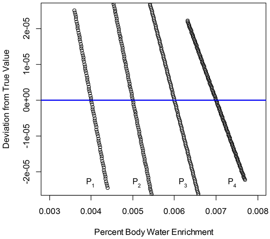
Numerical simulations validate the closed-form equations for A2(t)/A0(t) and A1(t)/A0(t) ratios. The y-axis shows the difference between the true value of A2/A0 and the value computed from Eq. (6) at various values of pX(t) (x-axis). The blue line is the y=0 line. Black circles on each curve are the values for one specific peptide, denoted as P1 through P4.
In Supporting Information, we provide a schematic and description of steps used in generating Figure 1. In Figure S1, we show the simulations of I0(t), I1(t), I2(t), and I3(t) as a function pX(t) for the peptide sequence, IQDAGLVLADALR, over the range of complete depletion of these mass isotopomers due to the labeling with deuterium. The closed-form equations determine pw values at which each mass isotopomer is completely depleted.
3.2. Tests on simulated rate constants
Using the R environment19, we implemented an approach to estimate DRC from the time-course of the A1(t)/A0(t) ratio using Eqs. (5), (2) and (1). We applied this method and compared it with the traditional method, which uses the time-course of I0(t) (obtained from complete isotope profile) to calculate the DRC. As the first test, we used the simulations because, in the simulations, we know the actual values of DRCs. We used the same 21706 DRCs (from the murine liver proteome) for each method.
For determinations from I0(t), the simulations were done using Eq. (1) for each DRC and adding to the actual time-course the errors sampled from the Laplace distribution (whose parameters were determined from the above-referenced data set of the murine liver)20. We then determined the simulated DRC using the noisy I0(t). In the following text, we refer to this as the traditional method.
For the A1(t)/A0(t) ratio, we assumed the Laplace distributed error as well. First, we computed the true value of A1(t)/A0(t). Then, we added Laplace distributed noise to the theoretical values. From the noisy-added A1(t)/A0(t) values, we determined pX(t) at every time point of labeling using Eq. (5). The pX(t) values were inserted into Eq. (2) to obtain the reconstructed time-course of I0(t). The time-course of the reconstructed I0(t) was used to determine DRC in this alternative method.
First, we checked if the two methods produced the same results when simulations used very small errors. Figure S2 of Supplementary Information shows the scatter plot of the rate constants produced by the two methods. The scaling parameter of Laplace distribution for errors was set to exp(−8). As expected from an exact solution, the scatter plot is the identity line.
When we increased the error parameter to make it equal to the estimations from the mouse liver data set (the scale parameter was exp(−4.14)), the rate constants computed by two methods showed some differences, Figure S3. We compared the calculated rate constants with the actual values. The scatter plot of the relative errors is shown in Figure S4. 19634 simulations using A1(t)/A0(t) ratio produced rate constant that agreed with actual values better than ten percent (of the actual values). The corresponding number from the I0(t) simulations was 9203. 8460 simulations produced better than ten percent agreement with the true values in both methods. Thus, assuming the same error distribution, A1(t)/A0(t) ratio method produced better results in these simulations.
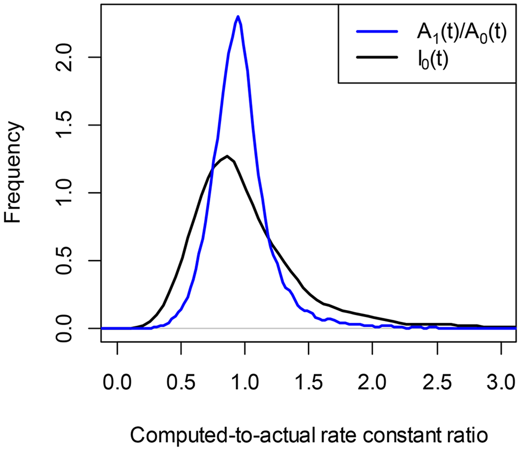
Figure 2 shows the scatter plot of the absolute values of the DRC errors calculated using I0(t) (y-axis) and A1(t)/A0(t) (x-axis) using actual data from the liver proteome. Less than 0.02% of the data were outside of the axis ranges. The red line is the identity line. For 74% of DRC, the absolute errors of simulated DRCs using I0(t) was higher than that from A1(t)/A0(t). The slope of the linear regression of the absolute value of the relative error on the correlations (between the “experimental” and theoretical time-course data) was −0.64 for A1(t)/A0(t) method and −0.32 for I0(t) method. Thus, for high values of the correlation (better agreement between the experimental data and theoretical fit), the relative error’s absolute value was smaller for both methods. Figure 3 shows the density plots of the computed-to-actual DRC ratios for the two methods. The data was filtered to keep only those that have corresponding correlations higher than 0.8. 89% and 65% of data passed the filtering for A1(t)/A0(t) and I0(t) methods, respectively. Both density functions have a mode near one, as expected. However, the method using A1(t)/A0(t) (blue curve) retained more data (after the filtering by correlation) and had a smaller standard deviation.
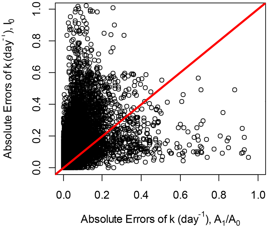
For many peptides, abssolute errors of rate constants obtained from the alternative approach were smaller than those from the traditional method. Scatter plot of absolute errors of rate constants estimations using A1(t)/A0(t) (x-axis) and I0(t) (y-axis). The red line is the line of identity.
3.3. Direct computations of rate constants of the murine liver proteome
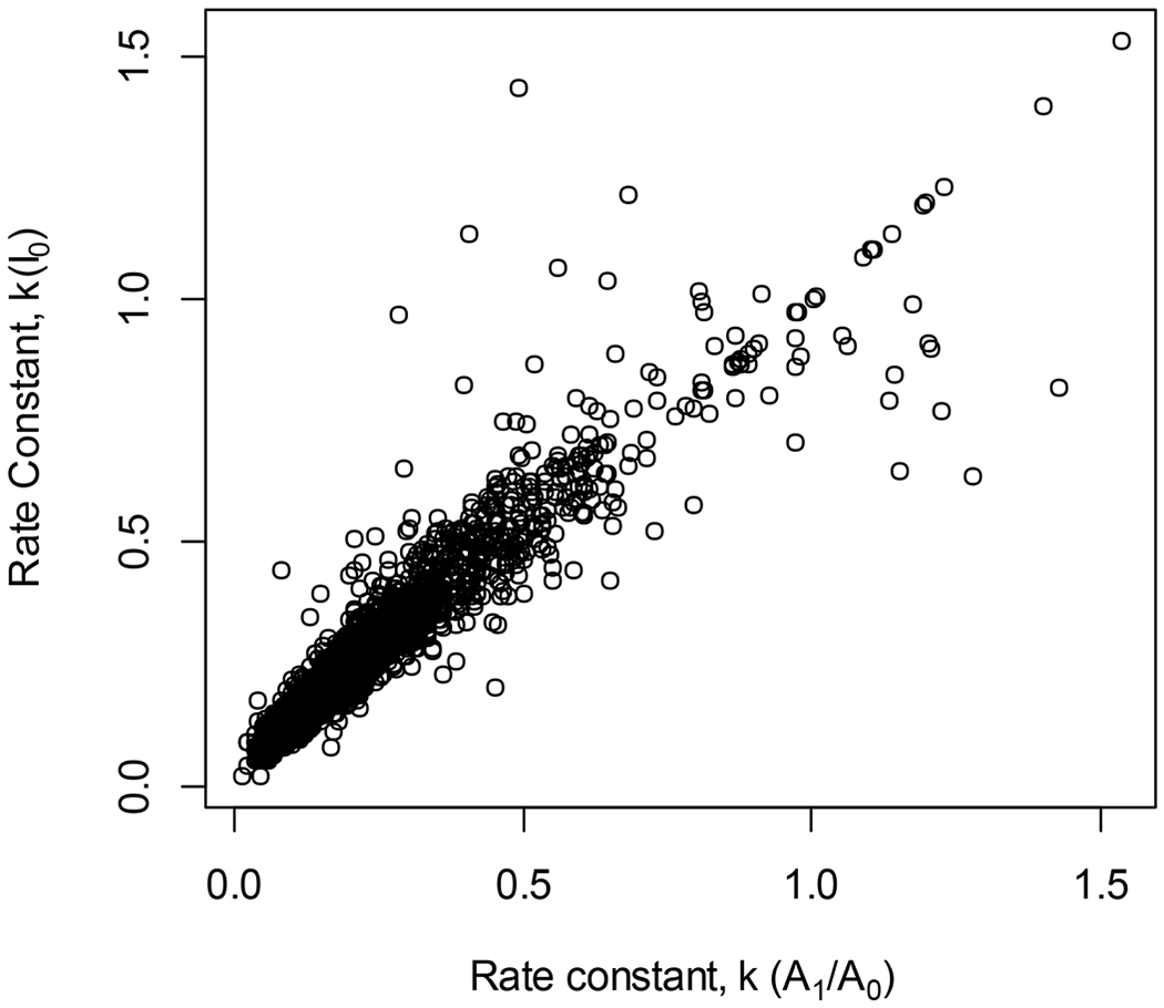
Next, we used both approaches to calculate the DRCs from the murine liver proteome. Out of the 21706 peptide entries, 6935 passed the correlation (0.975) and residual sum of squares (RSS) (0.001) filtering from both methods. 8059 and 11110 peptide entries passed the thresholds in the traditional and new methods, respectively. The scatter plot of the DRCs that passed more stringent filtering by both methods is shown in Figure 4. On the x-axis are the DRCs using two mass isotopomers, on the y-axis are the DRCs computed using the traditional method. In this figure, the rate constants were filtered to include only those that correlated with the experimental data with the Pearson correlation of 0.995 or better (from both methods).
4.1. Results and Discussions.
We have derived novel, closed-form equations that describe mass isotopomer dynamics of a peptide during deuterium incorporation from heavy water metabolic labeling. The equations provide mechanistic insights into the changes occurring in the isotope profiles. Eq. (3) shows that the time-course evolution of M1 mass isotopomer is contributed by two terms. The contribution from I0(0) increases over the duration of labeling, while the contribution from I1(0) decreases. The time-course of the M2 mass isotopomer, Eq. (6), is similar. It is determined by two terms: I1(t) and I0(t). It can also be expressed solely by the enrichment in the deuterium, pX(t), and the NEH value of a peptide. Using the derived equations, for every peptide, complete dynamics of the first four mass isotopomers can be generated from the values of I0(0), I1(0), I2(0), and I3(0). Figure S1 of Supplementary Information shows the dynamics of the mass isotopomers for the peptide sequence, IQDAGLVLADALR, generated theoretically. Previously, the generation of the mass isotopomer profiles required theoretical simulations of the relative abundances of the peptide, given the enrichment with the deuterium (and the NEH value). Using the closed-form equations, the dynamics is easily computed.
The developed equations can be used in various practical applications and to update analytical techniques currently used to analyze LC-MS data from metabolic labeling. Recently, Ilchenko and colleagues21 developed an approximation for determining NEH at the plateau enrichment. They approximated RAs by considering the first two mass isotopomers only. From Eq. (4), there is an exact formula between the raw abundances obtained from two mass isotopomers and the NEH value:
The approximate equation of Ilchenko did not contain the division of the third term in the denominator by
Formula based results provide several advantages. The estimation of RA of monoisotope at the plateau has been an integral part of the models for extracting protein turnover rates. Because of the known formula, we can now readily compute the exact form of the expected abundances for heavy mass isotopomers. For example, for the first and second heavy mass isotopomers, they are:
In previous approaches22, these quantities were obtained from simulations. The explicit form of I0 at the asymptote is well known and obtained from Eq. (1) by replacing (pX(t)+pH) with pW.
The newly derived equations provide an alternative approach to the estimation of rate constants. Currently, only 30-40% of all quantified peptides are viable for protein turnover estimations23. For the rest of the peptides, goodness-of-fit measures (RSS and the correlation between experimental data and theoretical fit) are below acceptable thresholds. One of the reasons for the low quality of quantification is the complexity of proteomes in mammalian samples. Even in high-resolution and mass accuracy mass analyzers, there are many co-eluting species that interfere with the peak detection and quantification of target peptides. When using many mass isotopomers, the chance of co-elution with at least one of them increases, and, through the normalization, the co-elution affects the RAs for all other mass isotopomers. One alternative approach, which the new closed-form equations allow, is to estimate the DRCs from two mass isotopomers only. As was noted by Anderson and coworkers16, the use of the two mass isotopomers, M0(t) and M1(t), is expected to be more accurate. For peptides, these two signals are, in general, the most abundant in the isotope profile. The time-course of A1(t)/A0(t) requires no normalization. Besides, a detailed analysis of spectral accuracy has found that Orbitrap mass spectrometers exhibit lesser errors in determining A1(t)/A0(t) ratios compared to those of the other mass isotopmers24. In Supplementary Information, we describe simulations and comparison of the errors in estimating I0(t) and A1(t)/A0(t) using the murine liver proteome data set. Figure S4 in Supplementary Information shows the comparison of the relative errors. Combining two methods increased the number of peptide entries with the errors of 5% or less (from the theoretical value) by 31%.
We have tested an alternative approach to estimating rate constants using only two mass isotopomers. At each time point of labeling, one estimates pX(t) using NEH and A1(t)/A0(t) ratio in Eq. (5). The calculated pX(t), NEH, and the theoretical value of I0(0) are inserted into Eq. (2) to reconstruct the time-course of I0(t). The time-course data is, then, used in non-linear least-square regression, Eq. (1), to estimate k. It is a numerically simple approach that uses the smallest number of mass isotopomers and does not employ approximations or expensive numerical calculations. The errors in the estimation of A1(t)/A0(t) and I0(t) in each case will determine which method to use for DRC. If both errors are small, they produce the same DRCs, Figure S2.
Figure 5 shows an example of DRC estimation using the A1(t)/A0(t) ratio. For the peptide sequence QIAAVMQR (cytoplasmic Aspartate aminotransferase), the non-linear least-squares fit to the experimental data of I0(t) (black circles) fails to converge. The fit to the data from A1(t)/A0(t) (blue diamonds) converges. The Pearson correlation between the fit and the experimental data was 0.99. The RSS was 0.0001. The calculated DRC was 0.11 day-1. The median of DRCs of 27 other peptides of the protein was 0.13 day−1.
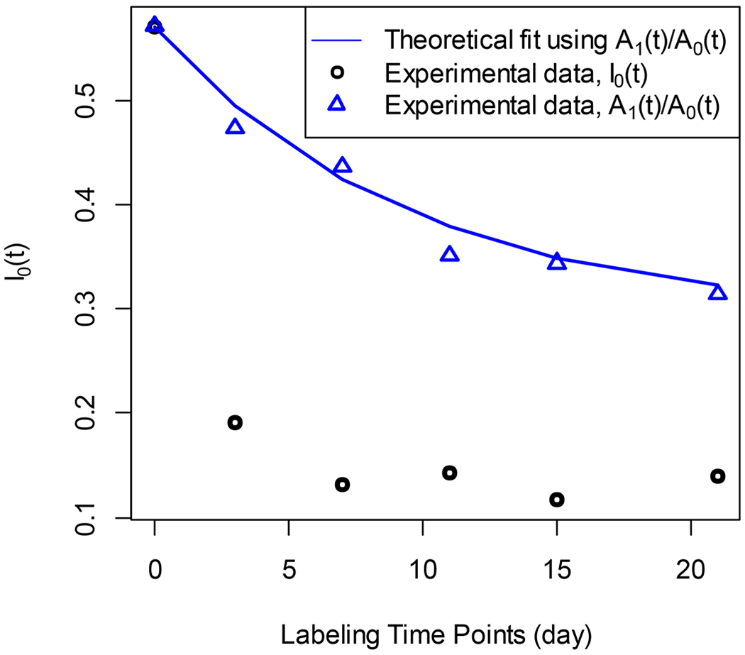
The alternative method computes the rate constant when the traditional method does not converge due to the contamination of the isotope profile of a peptide by a co-eluting species. The y-axis is the RA of the monoisotope, and the x-axis is the labeling duration.
The closed-form equations for extracting deuterium enrichment from the abundance of only two mass isotopomers will potentially be useful for efforts to quantify label incorporation using isotope distributions of fragment ions in MS2. We25 and others16 have shown that label incorporation is also exhibited in the MS2 spectra. However, most of the time, Orbitrap mass analyzers report truncated isotope profile (only two mass isotopomers) of fragment ions25, which is enough for the closed-form equations derived here.
Eqs. (4) and (6) uniquely define the time-course of the A2(t)/A1(t) ratio, as well. In the cases when a contaminant interferes with the monoisotopic peak of a peptide, the A2(t)/A1(t) ratio can be used for the analysis of the label incorporation.
In metabolic labeling using heavy water, deuterium atoms are incorporated into non-essential amino acids (NEAAs) and subsequently into proteins. There are a certain number of hydrogens (mostly in sidechains of NEAAs) in a peptide that are accessible to the deuterium in the heavy water. Thus, the label (deuterium) incorporation into a peptide is a function of the rate constant, NEH, pW, and the labeling duration. The estimation of the rate constant is sensitive to the accuracy of NEH determination. In principle, the NEH for each amino acid can be determined using GC-MS26. In practice, the NEH values of mouse amino acids, initially determined by Commerford and coworkers27 (using metabolic labeling with tritiated water), have been used for other species9. Eqs. (6) and (7) allow to uniquely determine NEH and pX(t) simultaneously from the ratios of the raw abundances of the first three mass isotopomers, Figure 1. For improved accuracy of the rate constant estimation and extending its applications to other species, it will be important to determine NEH values for each species, and preferably from LC-MS. The newly derived closed-form equations provide capabilities for such determinations, while still requiring only a partial isotope profile of a peptide.
Another practical application of the derived equations will be the use of their asymptotic forms to determine how many mass isotopomers are important in the analysis given the enrichment in the diet water, the number of exchangeable hydrogens, the natural isotope profile of a peptide. Currently, one cannot discard any of the high mass isotopomers a priori, because as the peptide is labeled with heavy water, the relative abundances of the high mass isotopomers increase. Using the derived equations, one obtains exact RAs of high mass isotopomers at the asymptote of labeling. An algorithm, then, can make an informed decision about which mass isotopomers to keep for the quantification. Keeping the most important (but a small number) of mass isotopomers is important for reducing the chances of interferences by the co-eluting contaminants. This application will help improve accuracy in the traditional method.
The developed closed-form equations are not specific to the labeling with deuterium. They apply to other atom-based labeling agents. For example, to describe the dynamics of RAs resulting from 15N labeling4, one needs to replace NEH with the number of accessible nitrogen sites, and pH with the natural abundance of 15N isotope. The pX(t) determined from the Eq. (5) will then be the enrichment of peptide with 15N.
The developments in this work complement our previous work on automating rate constant estimations13. That work developed an algorithm for peak detection and integration in a three-dimensional (m/z, elution time, and abundance) space. It then used the complete isotope profile of a peptide to determine the RA of the monoisotope. The time-course of RA during metabolic labeling was used to determine the rate constant. The process was automated to analyze data from high-throughput experiments. In that work, we did not employ any mass isotopomer algebra beyond calculating the RA of monoisotope from the complete isotope profile. In this work, we developed the closed-form equations for the first four mass isotopomers during the metabolic labeling with heavy water. The use of these equations in facilitating the data analysis is discussed.
Conclusion.
We present new closed-form equations that link the dynamics of the abundances of the first four mass isotopomers in metabolic labeling with heavy atoms. We show that the mechanistic insights gained into the complex mass isotopomer profiles can be used in practice to help in analyses proteome turnover. Thus, we show that only two mass isotopomers are enough to extract the deuterium enrichment precisely. Using the enrichment, one can reconstruct the RA of monoisotope and use it for rate constant estimation. The theoretical simulations prove the accuracy of the equations. Application to a real data set shows the relevance of the equations for improving DRC estimations in a practical setting.
From any triple of mass isotopomers, the equations allow simultaneous determinations of the number of sites that are accessible to heavy isotope atom and the enrichment in the heavy isotope. Equations for all four mass isotopomers can help to make an informed decision on the importance of the high mass isotopomers for proteome turnover.
Acknowledgements.
The research reported in this publication was supported in part by the NIGMS of the NIH under Award Number R01GM112044. The content is solely the responsibility of the author and does not necessarily represent the official views of the National Institutes of Health.
Abbreviations
| Eq | equation |
| FFT | fast-Fourier transform |
| GC | gas chromatography |
| LC-MS | liquid chromatography and mass spectrometry |
| LDLR | low-density lipoprotein receptor |
| MPE | molar percent excess |
| NEAA | non-essential amino acid |
| NEH | number of exchangeable hydrogens |
| RA | relative abundance |
| RSS | residual sum of squares |
Footnotes
Supporting Information. Supporting Note: The derivations, numerical validation of the closed-form equations, and tests using LC-MS data from heavy water metabolic labeling of mice. Figure S1: Profiles of the first four mass isotopomers of peptide sequence “IQDAGLVLADALR”. Figure S2: The scatter plot of the simulations of rate constants calculations using traditional and alternative approaches under small noise conditions. Figure S3: The scatter plot of the simulations of rate constants calculations using traditional and alternative approaches under experimental noise. Figure S4: Relative errors of rate constant estimations from two alternative approaches. Figure S5: The scatter plot of the relative errors of A1(t)/A0(t) and I0(t).
Conflict of Interest.
The author declares no conflict of interest.
References.
Full text links
Read article at publisher's site: https://doi.org/10.1021/acs.analchem.0c03343
Read article for free, from open access legal sources, via Unpaywall:
https://www.ncbi.nlm.nih.gov/pmc/articles/PMC8880304
Citations & impact
Impact metrics
Article citations
Flexible Quality Control for Protein Turnover Rates Using d2ome.
Int J Mol Sci, 24(21):15553, 25 Oct 2023
Cited by: 0 articles | PMID: 37958536 | PMCID: PMC10649227
Quantifying label enrichment from two mass isotopomers increases proteome coverage for in vivo protein turnover using heavy water metabolic labeling.
Commun Chem, 6(1):72, 17 Apr 2023
Cited by: 4 articles | PMID: 37069333 | PMCID: PMC10110577
FAMetA: a mass isotopologue-based tool for the comprehensive analysis of fatty acid metabolism.
Brief Bioinform, 24(2):bbad064, 01 Mar 2023
Cited by: 1 article | PMID: 36857618 | PMCID: PMC10025582
Software Tool for Visualization and Validation of Protein Turnover Rates Using Heavy Water Metabolic Labeling and LC-MS.
Int J Mol Sci, 23(23):14620, 23 Nov 2022
Cited by: 4 articles | PMID: 36498948 | PMCID: PMC9740640
TurnoveR: A Skyline External Tool for Analysis of Protein Turnover in Metabolic Labeling Studies.
J Proteome Res, 22(2):311-322, 27 Sep 2022
Cited by: 4 articles | PMID: 36165806 | PMCID: PMC10066879
Go to all (9) article citations
Data
Data behind the article
This data has been text mined from the article, or deposited into data resources.
BioStudies: supplemental material and supporting data
ProteomeXchange
- (1 citation) ProteomeXchange - PXD009493
Similar Articles
To arrive at the top five similar articles we use a word-weighted algorithm to compare words from the Title and Abstract of each citation.
Using Heavy Mass Isotopomers for Protein Turnover in Heavy Water Metabolic Labeling.
J Proteome Res, 20(4):2035-2041, 04 Mar 2021
Cited by: 4 articles | PMID: 33661639 | PMCID: PMC8167932
Protein turnover models for LC-MS data of heavy water metabolic labeling.
Brief Bioinform, 23(2):bbab598, 01 Mar 2022
Cited by: 5 articles | PMID: 35062023 | PMCID: PMC8921656
Review Free full text in Europe PMC
Quantifying label enrichment from two mass isotopomers increases proteome coverage for in vivo protein turnover using heavy water metabolic labeling.
Commun Chem, 6(1):72, 17 Apr 2023
Cited by: 4 articles | PMID: 37069333 | PMCID: PMC10110577
Dynamic Proteomics: In Vivo Proteome-Wide Measurement of Protein Kinetics Using Metabolic Labeling.
Methods Enzymol, 561:219-276, 17 Jul 2015
Cited by: 31 articles | PMID: 26358907
Review
Funding
Funders who supported this work.
NIGMS NIH HHS (1)
Grant ID: R01 GM112044
National Institute of General Medical Sciences (1)
Grant ID: R01GM112044
