Abstract
In this paper, we model the statistical properties of imaging exam durations using parametric probability distributions such as the Gaussian, Gamma, Weibull, lognormal, and log-logistic. We establish that in a majority of radiology procedures, the underlying distribution of exam durations is best modeled by a log-logistic distribution, while the Gaussian has the poorest fit among the candidates. Further, through illustrative examples, we show how business insights and workflow analytics can be significantly impacted by making the correct (log-logistic) versus incorrect (Gaussian) model choices.
Keywords: Probability distribution, Exam duration, Variations in practice, Simulation, Scenario modeling
Introduction
Providing diagnostic findings in a timely fashion is important to the cost-effective delivery of high-quality patient care. In diagnostic imaging, three key workstreams are the image acquisition, the image interpretation by the radiologist, and the timely communication of relevant results to the appropriate referring provider. Radiology administrators continuously monitor the timelines of these workstreams to adjust and improve operations [1–5].
Continuous monitoring is a difficult task because there are many different phases within each workstream that each contains natural variations giving rise to a distribution of possible values. Let us take for instance one such phase of time namely exam duration. Exam duration is the time it takes to acquire quality-controlled diagnostic images that are suitable for interpretation by radiologists. This important part of the image acquisition workstream influences the daily exam/patient capacity and therefore ultimately the efficient use of both fixed and variable assets within the radiology department. Exam duration can vary by patient demographics, by modality, by procedure type, and many other factors. This compels administrators to use representative values such as the mean and standard deviation to efficiently monitor and characterize performance. This approximation of the complex distribution of exam duration is a powerful way to condense a large set of data points to just two parameters. It is a common practice and a part of standard reporting and business analytics as well.
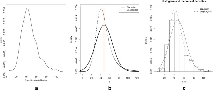
When using mean and standard deviation to represent a large set of values, we make a basic assumption that these values are normally distributed or, in other words, a standard Gaussian distribution. However, is this a valid assumption to make? Are exam durations best represented by a Gaussian distribution? In a vast majority of healthcare data sets (e.g., hospital length of stay, cost, survival times), it has been established that non-Gaussian distributions such as lognormal, Gamma, Weibull, and log-logistic are more suited and useful to glean insights. These non-Gaussian distributions are non-symmetric and right-skewed and have different statistical properties than Gaussian models. Figure 1 shows visually the shape of a representative sample of probability distributions. Figure 1a is the plot of a frequency distribution of exam duration observed for MRI of abdomen with and without contrast. Figure 1b shows two model distributions, namely Gaussian and log-logistic, with both having approximately the same mean and standard deviation as the data for MRI of the abdomen. Despite having the same mean and standard deviation, the shapes of the two distributions are different. Gaussian is symmetric at the mean, which implies that the probability of an exam finishing in under the mean (47 min) is the same as the probability of the exam taking more than the mean. However, we make a different interpretation with log-logistic. The probability of an exam finishing in under 47 min is higher than the probability that it will take longer than 47 min. Furthermore, log-logistic has a long right tail which is a closer approximation to the actual underlying data (see Fig. 1c). While the difference in statistical properties is visually observable, in this paper, we focus on taking a methodical approach to choosing a parametric probability distribution model to describe specific imaging procedures and establish how this can alter our interpretation of workflow analysis and improvements.
Fig. 1.
a The density distribution of the observed exam durations (in minutes) for MRI of the abdomen w/wo contrast. b The two theoretical distributions, namely Gaussian and log-logistic, with the same mean and standard deviation. The vertical line at x = 47 is the mean that divides the Gaussian into two symmetric halves. c The theoretical distributions laid on top of the actual data from (a) represented as a histogram
In particular, we make the following claims:
Distribution of exam durations, of a given radiology procedure, is non-Gaussian, and its statistical properties are better characterized by other parametric distributions such as Gamma, Weibull, lognormal, or log-logistic.
As a result, choice of Gaussian versus a non-Gaussian distribution model for exam durations can lead to significantly different business insights and workflow analysis.
Fitting a parametric probability distribution, to exam durations, is essential for stochastic sampling in computer simulation studies and to construct valid models of complex workflow interactions that would otherwise be cumbersome.
Data and Methods
Our data set was extracted from the Lahey Hospital and Medical Center (LHMC), Burlington, MA, Radiology Information System (RIS). LHMC is a mid-sized, independent academic medical center, which is the tertiary care hospital of an Integrated Care Delivery Network (IDN) centered in LHMC. Data over a period of 1 year (July 2015 to June 2016) was extracted with values for exam identifiers, modality type, procedure description, exam date, and exam duration. A similar data set was also extracted for the time period of July 2016 to June 2017.
At LHMC, between July 2015 and June 2016, a total of 253,047 imaging exams were performed at the Burlington site. Of these, 144,714 were outpatient exams spanning across 984 distinct imaging procedures. We restrict our analysis to outpatients because emergency room patients and inpatients are an inherently different population, in which more complex clinical needs prominently influence quantifiable exam characteristics. Our goal is to show that variations in exam durations exist even within one type of patient population and that we need intelligent models to capture these variations. Since outpatients are the majority among the three patient classes in the LHMC operation, we focus on outpatient procedures. The majority of these procedures generated only a few data points (577 procedures had 25 discrete exam instances or less). We decided to only choose procedures with 100 or more exams (since we need a sufficient number of data points to fit a model distribution), and this resulted in a final data set with 111,547 exams spanning 124 distinct procedures. Similarly, for the time period between July 2016 and June 2017, the final data set had 112,053 outpatient exams spanning across 125 distinct procedures. Throughout the remainder of this analysis, we will only use data from the first time period, July 2015 to June 2016, unless otherwise explicitly mentioned. Data from the second time period is only used in the “Results and Discussion” section to establish robustness of our results across time.
Table 1 shows the breakout of the data by modalities and the top two procedures. There are 22,227 exams that could not be classified under common diagnostic modalities (XR, CT, US, MR). Of these 12,985 (~ 60%) are screening mammograms. The other 9242 exams are spread across 17 procedures, consisting of advanced modalities such as positron emission computed tomography (PET CT), nuclear medicine (NM), and interventional radiology (IR) procedures.
Table 1.
Breakout of the data by modalities and the top two procedures within each modality
| Modalities and top two procedures | Number of procedures | Number of exams | Median exam duration (min) |
|---|---|---|---|
| Computed tomography (CT) | 20 | 13,562 | 16 |
| CT chest WO contrast | 3028 | 12 | |
| CT abdomen and pelvis W contrast | 2050 | 17 | |
| Magnetic resonance (MR) | 19 | 9859 | 44 |
| MRI brain W WO contrast | 2113 | 50 | |
| MRI abdomen W WO contrast | 1598 | 45 | |
| Ultrasound (US) | 15 | 21,158 | 22 |
| US retroperitoneal complete | 3191 | 19 | |
| US abdomen complete | 2643 | 24 | |
| X-ray (XR) | 52 | 37,155 | 13 |
| XR chest 2 VW | 8937 | 8 | |
| XR DXA bone density hip pelvis | 3788 | 15 | |
| Others | 18 | 22,227 | 17 |
| Mammogram screening tomosynthesis bilateral | 12,985 | 15 | |
| PET CT skull to mid-thigh | 2136 | 148 | |
| Grand total | 124 | 111,547 | 17 |
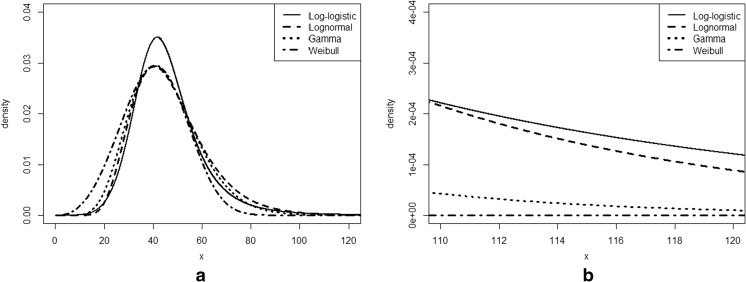
Next, in order to find the best fitting model for the data, we should first identify a candidate list. In this paper, a candidate is a pre-defined probability distribution function consisting of parameters that describe its functional form and shape. Our candidate list was chosen based on a survey of prior studies that have modeled healthcare data distributions, as well as their popular use in both academic literature and in non-healthcare domains [6–9]. Table 2 shows a list of candidates chosen, and Fig. 2 shows how the shapes of these distributions differ from one another. All the candidate models are unimodal, only take non-negative values (except Gaussian), and have long right tails. Further, they are all defined by exactly two parameters. Shapes of lognormal, Gamma, and Weibull are visually similar to each other and the main differentiator of these distributions can be seen near the tails (Fig. 2a). For a given coefficient of variation (defined as the ratio of standard deviation to the mean), lognormal has a longer tail than Gamma, which in turn has a longer tail than Weibull [8]. For the same coefficient of variation, the shape of log-logistic is different. Its peak is more prominent, but the density at the tail gradually becomes heavier than the other three (see Fig. 2b).
Table 2.
Candidate model distributions and their functional forms
| Name of PDF | Functional form | Parameters |
|---|---|---|
| Gaussian | μ and σ are the mean and standard deviation respectively | |
| Lognormal | σ and eμ are shape and scale parameters. Defined for x > 0. | |
| Log-logistic | α is the shape parameter and β is the scale parameters. x,α,β > 0. | |
| Gamma | α is the shape parameter and β is the inverse scale parameter. x,α,β > 0. | |
| Weibull | α is the shape parameter and β is the scale parameters. x,α,β > 0. |
Fig. 2.
a Plot showing the shapes of lognormal, Gamma, Weibull, and log-logistic distributions. b The distribution at the tails
With this material in hand, we will now proceed to define the methods we will use to determine the best fitting distribution model. We will first begin by identifying the best fit for one specific procedure namely MRI of abdomen w/wo contrast and then scale the methodology to all radiology procedures. We will represent the observed data for this procedure as and the distribution function as . Further the cumulative distribution function will be represented as .
Given the , we determine the Maximum Likelihood Estimates (MLEs) of the parameters of all the candidate distributions. Intuitively, MLE parameters are the most likely parameters of the model given the underlying data [10]. Once the MLE parameters are estimated, the model with the best fit is evaluated using goodness of fit statistics. For our analysis, we will use three commonly used goodness-of-fit measures namely Kolmogorov-Smirnoff (KS) statistic, Anderson-Darling (AD) statistic, and Akaike Information Criterion (AIC) [11].
The KS statistic is defined as and quantifies the supremum of the absolute difference between the empirical cumulative distribution, denoted as , obtained from the data , and the theoretical cumulative distribution, denoted as , of a model candidate. n stands for the number of data points available from the empirical data. When the two distributions are the same, Dn → 0 as n → ∞. That is, when n is large, we should see Dn as close to 0 as possible. The Anderson-Darling statistic defined as is the squared difference between and . It also uses a weighting function w(x) = (F(x)(1 − F(x))−1 that makes this statistic more sensitive to the differences in the tail [11]. Here again, if the two distributions are the same, then An → 0 as n → ∞. AIC has its origins in information theory. If is the maximum value of the likelihood function and m is the number of parameters in the model, then . Given a candidate set of parametric distributions, the preferred distribution is the one with minimum AIC. In general, smaller goodness-of-fit measures are preferred. It is important to note that this method will tell us which model is better relative to the others and does not say anything about the quality of fit in the absolute sense.
In this paper, we use R language and environment (version 3.3.1) for statistical computing (http://www.r-project.org/Vienna, Austria). In particular, we use the “fitdistrplus” package to fit parametric distributions (fitdistr()) to the data and evaluate the goodness of fit (gofstat()).
Results and Discussions
Discussion of results in this section ties back to the three claims we made in the “Introduction.”
Claim 1:
Distribution of exam durations, of a given radiology procedure, is non-Gaussian, and its statistical properties are better characterized by other parametric distributions such as Gamma, Weibull, lognormal, or log-logistic.
Table 3 shows the goodness-of-fit statistics of all the candidates (whose parameters are the maximum likelihood estimates) to TMR. It also shows the estimates for mean, median, and the 90th percentile (with 90% confidence intervals). Gaussian has the worst fit among all candidates. It overestimates the median and underestimates the tail at the 90th percentile. In fact, even the 90% confidence intervals fail to capture the median and 90th percentile value. As per all the three goodness-of-fit measures, log-logistic has the lowest value and therefore the best fit.
Table 3.
Goodness-of-fit for TMR, along with mean, median, and 90th percentiles with 90% confidence intervals
| Goodness of fit | ||||||
|---|---|---|---|---|---|---|
| Distribution | AD | KS | AIC | Mean (90% CI) | Median (90% CI) | 90th percentile (90% CI) |
| Gaussian | 19.42 | 0.096 | 13,526.53 | 46.94 (46.19, 47.69) | 47.08 (46.05, 47.92) | 68.42 (66.95, 69.52) |
| Lognormal | 6.38 | 0.065 | 13,478.05 | 47.20 (46.32, 48.30) | 43.97 (43.19, 44.96) | 70.96 (68.84, 73.53) |
| Log-logistic | 1.47 | 0.038 | 13,359.37 | 47.57 (46.40, 48.50) | 44.52 (43.56, 45.35) | 68.88 (66.68, 71.46) |
| Gamma | 4.77 | 0.049 | 13,391.60 | 47.00 (46.26, 47.83) | 45.09 (44.12, 46.03) | 69.02 (67.72, 70.82) |
| Weibull | 19.99 | 0.088 | 13,513.49 | 46.92 (46.25, 47.63) | 46.39 (45.52, 47.40) | 69.88 (68.52, 71.25) |
| T MR | 46.98 | 45 | 70 | |||
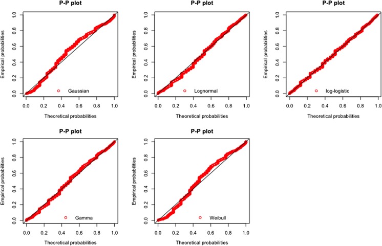
To further illustrate what these differences look like, we can use a P-P plot. In the P-P plot, for every point x, it plots , where and are cumulative distributions of a candidate model and respectively. If the model fits the data well, then as x goes from 0 → ∞, all points should fall along the diagonal line. Deviations from the diagonal indicate differences. In Fig. 3, we can see that Gaussian has one of the biggest deviations from the diagonal indicating that, not only at the median and 90th percentile but also across a spectrum of values, it fails to capture the patterns in underlying data. This is also the case with Weibull. Gamma, even though relatively better, also shows deviations. Among all candidates, log-logistic has the best fit. This visual plot matches closely with what we observe via the goodness-of-fit measures (also see Fig. 1c for a visual comparison of how the fitted distribution functions of the Gaussian and log-logistic models look like against the distribution of ).
Fig. 3.
Shows the P-P plot of the empirical distribution from TMR with the theoretical distributions of the candidate models with MLE parameters
We next repeat the same process for the procedure “MRI Abdomen W Wo Contrast” from the second time period (July 2016 to June 2017). Let us call this . As can be seen in Table 4, once again, Gaussian has the worst fit while log-logistic is the best choice among the candidates. This establishes the robustness of results across time.
Table 4.
Goodness-of-fit measures for TMR2
| Goodness of fit | |||
|---|---|---|---|
| Distribution | AD | KS | AIC |
| Gaussian | 30.65 | 0.11 | 13,003.98 |
| Lognormal | 21.74 | 0.10 | 13,123.61 |
| Log-logistic | 5.04 | 0.06 | 12,834.23 |
| Gamma | 16.37 | 0.08 | 12,954.03 |
| Weibull | 35.17 | 0.12 | 13,046.14 |
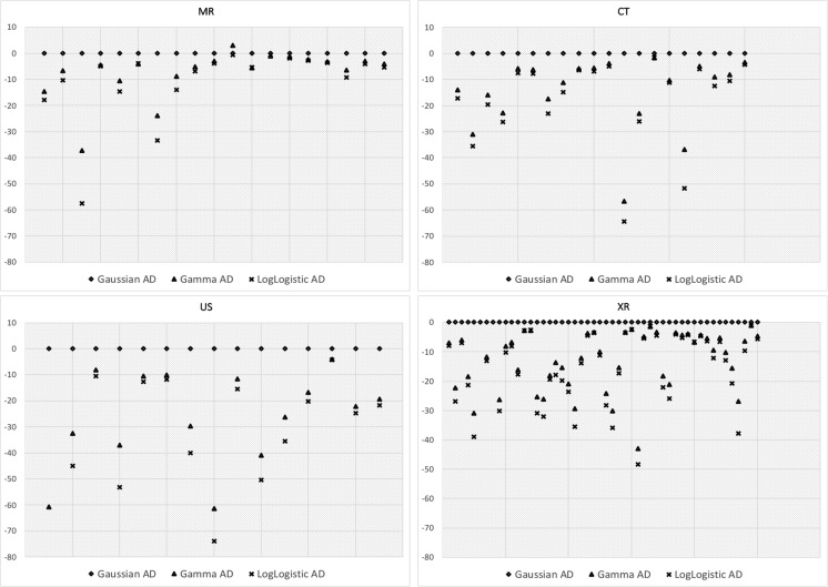
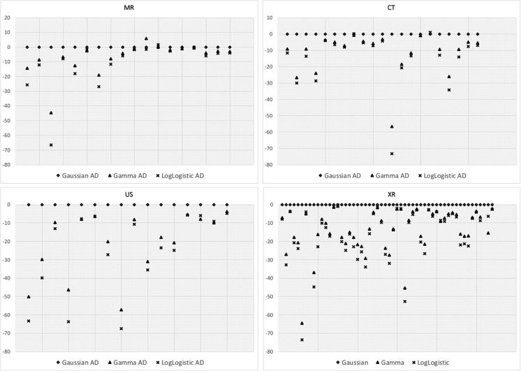
Having established that log-logistic is a better fit than Gaussian in one procedure, we can now look at the best fit across all radiology procedures. Figure 4 plots the comparison of the AD goodness-of-fit statistic of Gaussian, Gamma, and log-logistic model for every radiology procedure. Along the x-axis is the procedure and along the y-axis is the AD statistic relative to the Gaussian. That is, the y-axis represents the value of Gaussian AD–Candidate AD. A value of zero implies that the candidate distribution is as good as Gaussian, while a value less than zero implies that the candidate is better fit for that radiology procedure than the Gaussian.
Fig. 4.
Shows the AD statistic for specific radiology procedures categorized by modality. Along x-axis are the individual procedures and along y-axis is the AD statistic of candidate distributions relative to the Gaussian AD statistic. The smaller the statistic, or further down along the y-axis, the better is the fit
From Fig. 4, we observe the following: (1) in a majority of radiology procedures (across all modalities), Gaussian is the poorest fit among the candidate models and (2) log-logistic is the best fit and, even though Gamma lags behind log-logistic, it is still a much better fit than the Gaussian (Weibull and lognormal were removed to make the graphs more readable without compromising on our conclusions).
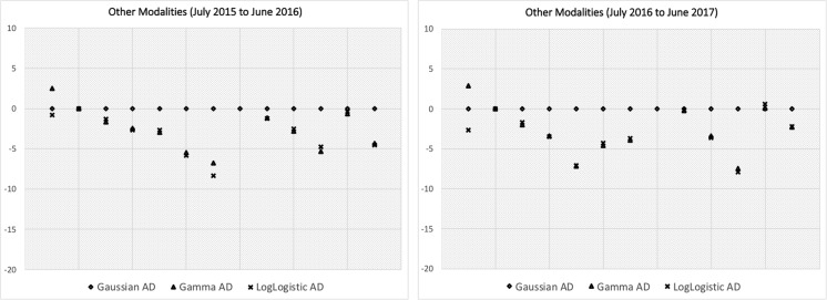
Figure 5 shows the same graph for data from the second time period (July 2016 to June 2017). Our conclusions regarding the model fit remain the same, thus establishing the robustness across time periods. Figure 6 shows the same graph for procedures that fall under other modalities and we can make similar conclusions.
Fig. 5.
Shows the same information as in Fig. 4 but for a different time period between July 2016 and June 2017
Fig. 6.
Shows the same information as in Figs. 4 and 5, but for procedures in modalities other than CT, MR, XR and US, across two different time periods
Claim 2:
As a result, choice of Gaussian versus a non-Gaussian distribution model for exam durations can lead to significantly different business insights and workflow analysis.
In order to prove Claim 2, let us set up the following experiment. On a typical weekday at LHMC, approximately 110 outpatient CT exams are performed. Over the years, the CT department underwent many workflow changes but still maintained the exam slot size at 20 min. So, if we wanted to increase capacity at this facility, we should first do an analysis of how much time is currently available within the workflow that can then inform us on how much additional capacity can be absorbed. Some exams take longer than the allocated slot size (20 min) to complete, leading to tardiness of the process, and some finish quicker, leading to waste in the process. Within the existing workflow, we want to estimate waste–tardy (i.e., waste over and above tardiness) per day that in turn can tell us how many additional exam slots per day could potentially be accommodated. The authors acknowledge that in actual practice, recovery of wasted time would require prospective change in scheduling practice, but for the purposes of this thought exercise, we ignore the complexity of scheduling.
Table 5 shows how much additional capacity is theoretically available per day by fitting the underlying exam duration data (for each CT procedure) using both a Gaussian distribution and a log-logistic distribution. The type of procedure performed in each slot is simulated based on the frequency of these procedures in the data. We can see that under the assumption of Gaussian, we underestimate, by 4 slots per day, the additional available capacity. This result manifests because the Gaussian distribution often overestimates the number of procedures that run long. Assuming approximately $650 global revenue per CT exam, this difference is as much 4 × $650 × 260 = $656,000 per year (260 is the number of weekdays in a year). Thus, we see the impact of identifying the underlying data using one type of distribution versus another and particularly how a Gaussian assumption can underestimate revenue opportunities.
Table 5.
Using both Gaussian and log-logistic model, the table shows how many more CT outpatient exam slots can be added per day at [hospital name - removed for review]
| Log-logistic model | Gaussian model | |
|---|---|---|
| # Outpatient CT exams/day at [hospital name - removed for review] | 110 | 110 |
| Exam slot size | 20 min | 20 min |
| Tardy = expected duration in minutes that go over the slot size (90% CI) | 219 (112, 391) | 275 (163, 435) |
| Waste = expected duration in minutes that finish within the slot size (90% CI) | 526 (427, 638) | 500 (373, 674) |
| Expected waste–tardy in minutes | 307 | 225 |
| Expected (waste–tardy) ÷ 20 min | 15 slots | 11 slots |
In practice, if one were to use the Gaussian model to describe the patient exams, then it would be easy to conclude that a large number of exams exceed the slot length, and therefore, a more appropriate slot might be 25 min. This overestimation of the number of exams that run late is a practical manifestation of choosing the inappropriate statistical model.
Claim 3:
Fitting a parametric probability distribution, to exam durations, is essential for stochastic sampling in computer simulation studies and to construct valid models of complex workflow interactions that would otherwise be cumbersome.
Let us again look at this claim using an illustrative example. Before we begin with an example, it is important to note the following. As mentioned before, parametric distribution models are a powerful way to compress a large set of data points using only a few parameters. In the case of a log-logistic distribution, its parameters are α and β. It can be shown that α is in fact the median of the distribution, and β is the dispersion parameter, i.e., increasing or decreasing β decreases or increases the standard deviation (and other dispersion metrics) [9].
Further, at large scale, computer simulation of radiology workflow is key to understanding improvement opportunities, and parametric distributions of processing times (such as exam duration) are usually taken as an input [9, 12–14]. Parametric distributions become even more relevant when one needs to model complex tasks (or decisions) within the workflow appropriately [9]. Let us take, for example, the decision a modality manager or a technologist makes when their day is running behind schedule. In LHMC, there are three MR machines on the main campus, and when an exam runs much longer than expected on any given machine, a decision is made to move the next exam scheduled for that machine to a different machine. This is a common occurrence and is often done to reduce subsequent patient wait times and to keep the workflow moving forward. How do you capture this in a simulation?
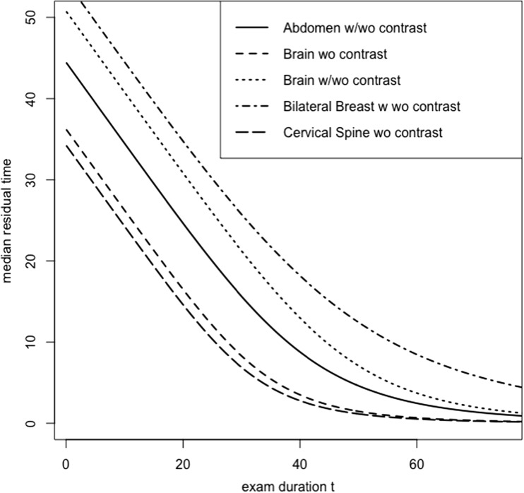
When exam durations are modeled as a log-logistic distribution, there is an easy way to obtain estimates of residual times. That is, given an exam has already taken t minutes, the additional time required to finish the exam is called the residual time to complete. For log-logistic, the median residual time can be shown to be . That is, if an exam has taken t minutes so far, this equation gives the median time remaining to complete the exam. Notice that when t = 0, i.e., at the start of the exam, the residual time is α, which is precisely the median of exam durations. Figure 7 shows the median residual times for the top 5 MR procedures. We can provide this function as an input to the computer simulation (refer to [9] for derivations of mean residual time, median residual time, and residual times at other quantiles). For example, if a patient has already arrived and has been waiting for 30 min or longer, then the decisions made by the staff on ground can be modeled by, say, if the median residual time to complete the current exam is more than 30 min then re-schedule the waiting patient to a different machine. Further, this decision can be re-simulated with multiple if then conditions to identify an ideal strategy to switch exams to different machines.
Fig. 7.
Shows the median residual time for the top 5 MR procedures. x-axis is the current duration of exam in minutes, and y-axis shows the median residual time remaining to complete the exam
Even though this is an illustrative example, we can see how parametric distribution models and their functional forms (see Table 2) can be used to create valid models of various workflow activities and decisions. Similarly, other candidates such as Gamma, lognormal, and Weibull also each have distinct properties that can be useful for workflow simulation models. Hence, the choice of a good parametric distribution candidate, for exam durations, depends not only on the best fit but also on how flexible the candidate is to create valid simulation models.
Conclusions
In this paper, we have established that distributions of imaging exam durations are non-Gaussian which is contrary to the predominant reporting practice in most radiology departments (using mean and standard deviation). We have shown that there are other two-parameter distributions that can fit the underlying data patterns better, and in particular, the log-logistic distribution was shown to be the best fit in a majority of imaging procedures. Also, we have shown that this pattern in data is consistent across time periods and across multiple modalities and procedures. Further, through illustrative examples, we have shown that an incorrect choice of distribution model can have a significant impact on workflow and business insights, and the correct choice of parametric distributions can lend itself well to creating valid models of complex activities and decisions within a radiology workflow.
One of the major limitations of this work is that the analysis was done on data from one institution only. However, the methodology described here is universal and can be used on any other data set consisting of radiology exam durations. Further, even though our paper focused on only one turnaround time, exam duration, the methodology is transferrable to all other phases of times (e.g., patient wait times, report turnaround times, etc.).
Footnotes
Publisher’s note
Springer Nature remains neutral with regard to jurisdictional claims in published maps and institutional affiliations.
Contributor Information
Usha Nandini Raghavan, Phone: 781-583-8086, Email: [email protected].
Christopher S. Hall, Email: [email protected]
Ranjith Tellis, Email: [email protected].
Thusitha Mabotuwana, Email: [email protected].
Christoph Wald, Email: [email protected].
References
- 1.Lloyd HD, Holsenback JE. The use of six sigma in health care operations: application and opportunity. Acad Health Care Manag J. 2006;2:41–49. [Google Scholar]
- 2.Nitrosi A, Borasi G, Nicoli F, Modigliani G, Botti A, Bertolini M, Notari P. A filmless radiology department in a full digital regional hospital: quantitative evaluation of the increased quality and efficiency. J Digit Imaging. 2007;20:140–148. doi: 10.1007/s10278-007-9006-y. [DOI] [PMC free article] [PubMed] [Google Scholar]
- 3.Towbin AJ, Iyer SB, Brown J, Varadarajan K, Perry LA, Larson DB. Practice policy and quality initiatives: decreasing variability in turnaround time for radiographic studies from the emergency department. Radiographics. 2013;33(2):361–371. doi: 10.1148/rg.332125738. [DOI] [PubMed] [Google Scholar]
- 4.Boland GW, Halpern EF, Gazelle GS. Radiologist report turnaround time: impact of pay-for-performance measures. AJR Am J Roentgenol. 2010;195(3):707–711. doi: 10.2214/AJR.09.4164. [DOI] [PubMed] [Google Scholar]
- 5.Gunn ML, Lehnert BE, Maki JH, Hall C, Amthor T, Senegas J, Beauchamp NJ: Using modality log files to guide MR protocol optimization and improve departmental efficiency. Radiological Society of North America (RSNA) Annual Meeting 2015. Health Services, Policy and Research (Medical/Practice Management) SSM12-02. 2015.
- 6.Gardiner JC, Luo Z, Xiaoqin T, Ramamoorthi RV. Fitting heavy-tailed distributions to health care data by parametric and Bayesian methods. J Stat Theory Pract. 2013;8(4):619–652. doi: 10.1080/15598608.2013.824823. [DOI] [Google Scholar]
- 7.Marazzi A, Paccaud F, Ruffieux C, Beguin C. Fitting the distributions of length of stay by parametric models. Med Care. 1998;36:915–927. doi: 10.1097/00005650-199806000-00014. [DOI] [PubMed] [Google Scholar]
- 8.Silva E, Lisboa P: Analysis of the characteristic features of the density functions for Gamma, Weibull and log-normal distributions through RBF network pruning with QLP. Proceedings of the 6th WSEAS Int. Conf. on Artificial Intelligence, Knowledge Engineering and Data Bases, 2007;6: pp 223–228
- 9.Clarke DE, Muhammad E. Some useful properties of log-logistic random variables for healthcare simulation. Int J Stat Med Res. 2015;4:79–86. doi: 10.6000/1929-6029.2015.04.01.9. [DOI] [Google Scholar]
- 10.Levy R: Probabilistic models in the study of language, chapter 4–parameter estimation, under preparation, http://www.mit.edu/~rplevy/pmsl_textbook/chapters/pmsl_4.PDF. Last access - Nov 15, 2016
- 11.Evans D, Drew J, Leemis L. The distribution of the Kolmogorov–Smirnov, Cramer–von Mises, and Anderson–Darling test statistics for exponential populations with estimated parameters. Commun Stat Simul Commun. 2008;37:1396–1421. doi: 10.1080/03610910801983160. [DOI] [Google Scholar]
- 12.Ramakrishnan S, Nagarkar K, Degennaro M, Srihari K, Courtney AK: A study of CT scan area of a healthcare provider. In: Ingalls RG, Rossetti MD, Smith JS, Peters BA Eds. Proceedings of the 2004 Winter Simulation Conference, 2005:2: pp 2025–2031. 10.1109/WSC.2004.1371565
- 13.Granja C, Almada-Lobo B, Janela F, Seabra J, Mendes A. An optimization based on simulation approach to the patient admission scheduling problem: diagnostic imaging department case study. J Digit Imaging. 2014;27(1):33–40. doi: 10.1007/s10278-013-9626-3. [DOI] [PMC free article] [PubMed] [Google Scholar]
- 14.Wang L: An agent-based simulation for workflow in emergency department. Systems and Information Engineering Design Symposium. Charlottesville, VA, 2009, pp 19–23.


