Abstract
Free full text

BIONIC: biological network integration using convolutions
Abstract
Biological networks constructed from varied data can be used to map cellular function, but each data type has limitations. Network integration promises to address these limitations by combining and automatically weighting input information to obtain a more accurate and comprehensive representation of the underlying biology. We developed a deep learning-based network integration algorithm that incorporates a graph convolutional network framework. Our method, BIONIC (Biological Network Integration using Convolutions), learns features that contain substantially more functional information compared to existing approaches. BIONIC has unsupervised and semisupervised learning modes, making use of available gene function annotations. BIONIC is scalable in both size and quantity of the input networks, making it feasible to integrate numerous networks on the scale of the human genome. To demonstrate the use of BIONIC in identifying new biology, we predicted and experimentally validated essential gene chemical–genetic interactions from nonessential gene profiles in yeast.
High-throughput functional genomics projects produce massive amounts of biological data for thousands of genes, often represented as gene–gene interaction networks, which link genes or proteins of related function1. These functional interaction networks have varying rates of false-positives and -negatives and integrating them promises to generate more accurate and complete functional networks. However, the diversity of experimental methods makes unifying this information a major challenge.
Existing network integration methods have not yet solved this problem. For example, many integration algorithms produce networks that retain only global topological features of the original networks, which can be at the expense of important local relationships2–5, whereas others fail to effectively integrate networks with partially disjoint node sets6,7. Some methods incorporate too much noise in their output, for instance by using more dimensions than necessary to represent their output, which can be detrimental to gene function and functional interaction prediction quality2–6. Most data integration approaches do not scale in the number of networks or in the size of the networks required for real world settings4,6,8. Supervised methods have traditionally been the most common network integration approach5,8–10 and, while highly successful, they require labeled training data to optimize their predictions of known gene functions, which may not be available. Moreover, annotations can be biased and limited, working only with known functional descriptions and reinforcing the existing understanding of gene relationships rather than identifying new ones.
To address the potential bias of supervised approaches, unsupervised biological network integration methods have recently been expl ored2–4,6,7,11. Theoretically, unsupervised network integration methods can provide a number of desirable features such as automatically retaining high-quality gene relationships and removing spurious ones, inferring new relationships based on the shared topological features of many networks in aggregate and outputting comprehensive results that cover the entire space of information associated with the input data, all while remaining agnostic to any particular view of biological function. However, practically, unsupervised methods still face challenges, such as scalability. Recently, new unsupervised data representation methods have been developed that focus on learning compact features over networks12,13. However, this approach produces general-purpose node features that are not necessarily optimal for the task of interest. Advances in deep learning have addressed this shortcoming with the development of the graph convolutional network (GCN), a general class of neural network architectures that are capable of learning features over networks14–17 in a scalable manner. Compared to general-purpose node feature learning approaches12,13, GCNs have substantially improved performance for a range of general network tasks14,17.
Here we present a general, scalable deep learning framework for network integration called BIONIC (Biological Network Integration using Convolutions), which uses GCNs to learn a single, unified feature vector for each gene, given many different input networks. BIONIC addresses the aforementioned limitations of existing integration methods and produces integration results that accurately reflect the underlying network topologies and capture functional information. To demonstrate the use of BIONIC, we integrate three diverse, high-quality gene and protein interaction networks, to obtain integrated gene features that we compare to a range of function prediction benchmarks. We analyze our findings in the context of those obtained from a wide range of integration methodologies12,17, and we show that BIONIC features perform well at both capturing functional information and scaling in terms of the number of networks and network size, while maintaining gene feature quality. Finally, we applied BIONIC network integration toward the analysis of chemical–genetic interactions18, which allowed us to make predictions about the cellular targets of previously uncharacterized bioactive compounds.
Results
BIONIC architecture
BIONIC uses the GCN neural network architecture to learn optimal gene (protein) interaction network features individually and combines these features into a single, unified representation for each gene (Fig. 1). First, the input data, if not already in a network format, are converted to networks (for example, by gene expression profile correlation) (Fig. 1a). Each input network is then run through a sequence of GCN layers (Fig. 1b) to produce network-specific gene features. The number of GCN layers used (three layers in our experiments: Methods and Supplementary Data File 1) determines the size of the neighborhood (that is, genes directly connected to a given gene) used to update the gene features14, where one layer would use only the gene’s immediate neighbors, two layers would use the second order neighborhood and so on. Residual connections are added from the output of each network-specific GCN layer in the sequence to the output of the final GCN in the sequence (Extended Data Fig. 1). This allows BIONIC to learn gene features based on multiple neighborhood sizes rather than just the final neighborhood, while additionally improving training by preventing vanishing gradients19. The network-specific features are then summed through a stochastic gene dropout procedure to produce unified gene features that can be used in downstream tasks, such as functional module detection or gene function prediction. To optimize the functional information encoded in its integrated features, BIONIC must have relevant training objectives that facilitate capturing salient features across multiple networks. Here, BIONIC uses an unsupervised training objective, and if some genes have functional labels (such as complex, pathway or bioprocess membership annotations), BIONIC can also use these labels to update its learned features through a semisupervised objective.
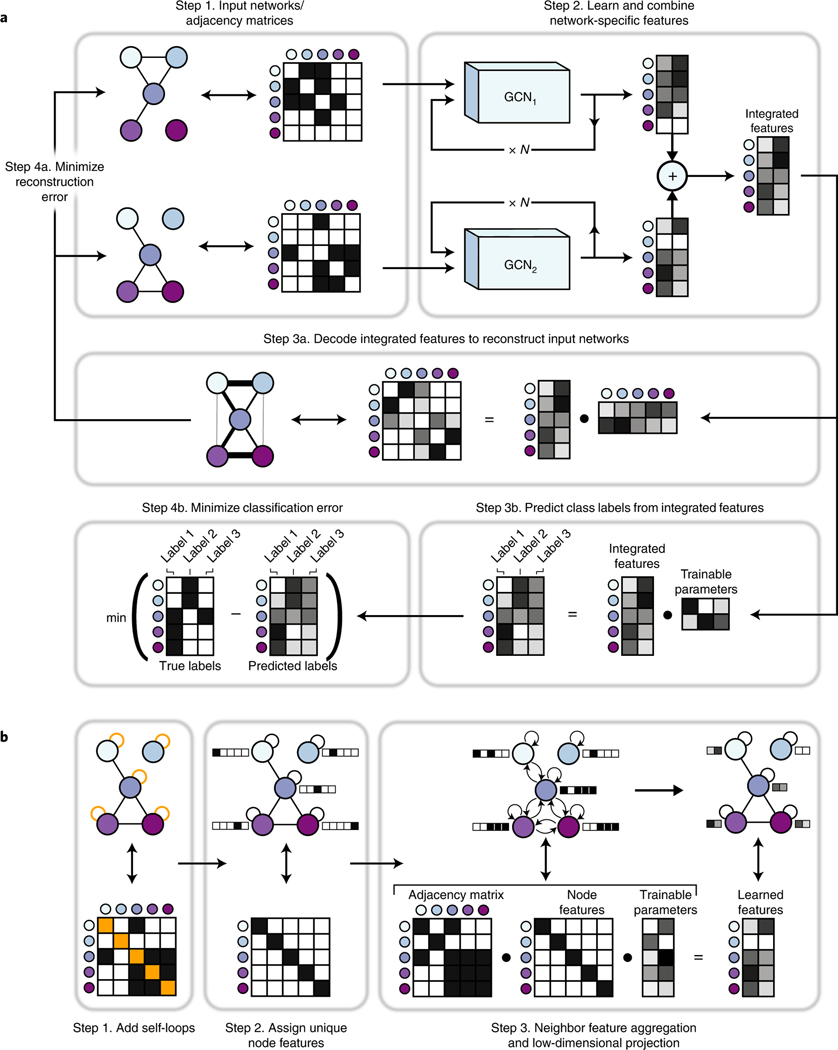
a, BIONIC integrates networks as follows: Step 1. Gene interaction networks input into BIONIC are represented as adjacency matrices. Step 2. Each network is passed through a graph convolution network (GCN) to produce network-specific gene features that are then combined into an integrated feature set that can be used for downstream tasks such as functional module detection. The GCNs can be stacked multiple times (denoted by
For the unsupervised objective, BIONIC uses an autoencoder design and reconstructs each input network by mapping the integrated gene features to a network representation (decoding) and minimizing the difference between this reconstruction and the original input networks. By optimizing the fidelity of the network reconstruction, BIONIC forces the learned gene features to encode as much salient topological information present in the input networks as possible, which reduces the amount of spurious information encoded. Indeed, for a set of three yeast networks20–22, inputting these networks into BIONIC individually tends to produce features with higher performance on several benchmarks compared to the original network format (Extended Data Fig. 2). This is likely due to the tendency for BIONIC to progressively embed related genes closer together during the training process, while ensuring unrelated genes remain far apart (Extended Data Fig. 3). By reconstructing the input networks, BIONIC is also trained to model the latent factors from each network that will best reconstruct all input networks.
For the semisupervised objective, BIONIC predicts labels for each gene using the integrated gene features and then updates its weights by minimizing the difference between the predictions and a set of user-specified ground-truth functional labels. Here, BIONIC performs multi-label classification, where a given gene may be assigned more than one class label. BIONIC ignores the classification error for any genes lacking ground-truth labels and so is able to incorporate as much (or as little) labeled information as is available. The semisupervised classification objective is used in conjunction with the unsupervised network reconstruction objective when gene labels are available, and the unsupervised objective is used on its own when no gene labels are available.
Evaluation criteria
For the following analyses, we assessed the quality of the input networks and network integration method outputs using three evaluation criteria: (1) gene coannotation prediction; (2) gene module detection and (3) supervised gene function prediction. First, we used an established precision-recall evaluation strategy22,23 to determine how well gene– gene relationships produced by the given method overlapped with gene pairs coannotated to the same term in a particular functional standard. Second, we evaluated the capacity of each method to produce biological modules by comparing clusters computed from the output of each method to known modules such as protein complexes, pathways and biological processes. These two evaluations measure the intrinsic quality of the outputs generated by the integration methods, that is without training any additional models on top of the outputs. Finally, the supervised gene function prediction evaluation determines how discriminative the method outputs are for predicting known gene functions. Here, a portion of the genes and corresponding labels (known functional classes such as protein complex membership) were held out and used to evaluate the accuracy of a support vector machine (SVM) classifier24, which is trained on the remaining gene features, output from the given integration method, to predict the held-out labels7. This constitutes an extrinsic evaluation, indicating how effectively the method outputs can be used in conjunction with an additional classification model.
In the following experiments, to ensure a fair choice of hyperparameters across BIONIC and the integration methods we compared to, we performed a hyperparameter optimization step using an independent set of Schizosaccharomyces pombe networks as inputs25–27 and a set of Gene Ontology (GO) curated pombe protein complexes28 for evaluation. The best performing hyperparameters for each approach were used (Methods).
Evaluation of BIONIC features and input networks
We first used the unsupervised BIONIC to integrate three diverse yeast networks: a comprehensive network of correlated genetic interaction profiles (4,529 genes, 33,056 interactions)22, a coexpression network derived from transcript profiles of yeast strains carrying deletions of transcription factors (1,101 genes, 14,826 interactions)21 and a protein–protein interaction network obtained from an affinity-purification mass-spectrometry assay (2,674 genes, 7,075 interactions)20, which combine for a total of 5,232 unique genes and 53,351 unique interactions (Fig. 2 and Supplementary Data File 2). Compared to the input networks, BIONIC integrated features have equivalent or superior performance on all evaluation criteria over three different functional benchmarks: IntAct protein complexes29, Kyoto Encyclopedia of Genes and Genomes (KEGG) pathways30 and GO Biological Processes28 (Fig. 2a and Supplementary Data File 3). The coannotation and module detection benchmarks contain between 1,786 and 4,170 genes overlapping the integration results. The module detection benchmarks define between 107 and 1,809 modules. The IntAct, KEGG and GO Biological Process gene function prediction benchmarks cover 567, 1,770 and 1,211 genes overlapping the integration results, and 48, 53 and 63 functional classes, respectively (Supplementary Data File 2). As an additional test, BIONIC produces high-quality features that accurately predict a diverse set of yeast biological process annotations per gene22 (Fig. 2b). Some categories in this last test do better than others. These performance patterns were mirrored in the individual input networks, indicating that this is the result of data quality, rather than method bias.
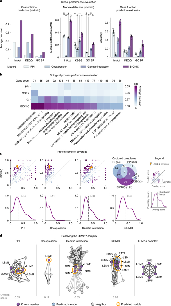
a, Functional evaluations for three yeast networks, and unsupervised BIONIC integration. Data are presented as mean values. Error bars indicate the 95% confidence interval for
We observed that features obtained through BIONIC network integration often outperformed the individual input networks at capturing functional modules (Fig. 2a) and captured more modules (Fig. 2c and Supplementary Data File 4), demonstrating the use of the combined features over individual networks for downstream applications such as module detection. Here we treated the network adjacency profiles (rows in the adjacency matrix) as gene features. We then examined how effectively the input networks and integrated BIONIC features captured known protein complexes, by matching each individual known complex to its best-matching predicted module and quantifying the overlap (Fig. 2c). We then compared the overlap scores from each network to the BIONIC overlap scores to identify complexes where BIONIC performs either better or worse than the input networks. Of 344 protein complexes tested, BIONIC strictly improved 196, 309 and 222 complex predictions and strictly worsened 82, 17 and 98 complex predictions compared to the input protein–protein interaction, coexpression and genetic interaction networks, respectively. The distributions of complex overlap scores for each dataset indicate that BIONIC predicts protein complexes more accurately than the input networks on average. Indeed, if we use an overlap score of 0.5 or greater to indicate a successfully captured complex, the integrated BIONIC features, containing information from three networks, capture 121 complexes, compared to 88, 3 and 74 complexes for the individual protein–protein interaction, coexpression and genetic interaction networks, respectively (Fig. 2c). We also repeated this module analysis while optimizing the clustering parameters on a per-module basis, an approach that tests how well each network and BIONIC perform at capturing modules under optimal clustering conditions for each module. Here too, the integrated BIONIC features capture more modules and with a greater average overlap score than the individual input networks (Extended Data Figs. 4 and and55 and Supplementary Data File 5).
To better understand how BIONIC is able to improve functional gene module detection compared to the input networks, we examined the LSM2–7 complex, which was identified in our module detection evaluation (Fig. 2a) as an example to show how BIONIC effectively combines gene–gene relationships across different networks and recapitulates known biology. The LSM2–7 complex localizes to the yeast nucleoli and is involved in the biogenesis or function of the small nucleolar RNA SNR5 (ref. 31). LSM2–7 is made up of the protein products of six genes: LSM2, LSM3, LSM4, LSM5, LSM6 and LSM7. We found that the cluster that best matched the LSM2–7 complex in each input network only captures a subset of the full complex (Supplementary Data File 4). The BIONIC module, however, contains five out of six members of the LSM2–7 complex, along with two additional members: LSM1 and PAT1, which are functionally associated with the LSM2–7 complex32. The missing member, LSM5, is in the local neighborhood of the cluster in the BIONIC feature space. We examined the best-matching clusters and their local neighborhood, consisting of genes that show a direct interaction with predicted members of the LSM2–7 complex, in the input networks, and in a profile similarity network obtained from the integrated BIONIC features of these networks (Fig. 2d). We found that both the PPI and genetic interaction networks captured two members of the LSM2–7 complex, with two additional members in the local neighborhood. The coexpression network only identified one complex member, and the local neighborhood of the best-matching module did not contain any additional known complex members. Finally, BIONIC used the interaction information across input networks to better identify the LSM2–7 module, with the addition of two functionally related proteins. This analysis demonstrates the use of BIONIC for identifying meaningful biological modules by effectively combining information across input networks. Indeed, when we optimized the module detection procedure to specifically resolve the LSM2–7 complex, we found that BIONIC was able to capture the complex with a higher overlap score (0.83) than any of the input networks (0.33, 0.17 and 0.50 for the PPI, coexpression and genetic interactions networks, respectively), and it outperformed other integration methods (0.43, 0.22, 0.44, 0.60 and 0.68 for the Union, iCell, deepNF, Mashup and multi-node2vec methods, respectively) (Supplementary Data File 5).
We also performed an analysis to examine how BIONIC features encode the input networks and found that the input networks are generally encoded uniformly across feature dimensions (Supplementary Note 1 and Extended Data Fig. 6).
Evaluation of BIONIC and established unsupervised integration methods
We compared network integration results from the unsupervised BIONIC (Fig. 2) to those derived from several different established integration approaches: a naive union of networks (Union), a nonnegative matrix tri-factorization approach (iCell)2, a deep learning multi-modal autoencoder (deepNF)11, a low-dimensional diffusion state approximation approach (Mashup)7 and a multi-network extension of the node2vec (ref. 13) model (multi-node2vec)33 (Fig. 3). These unsupervised integration methods cover a wide range of methodologies and the main possible output types (networks for Union and iCell, features for deepNF, Mashup and multi-node2vec). BIONIC performs as well as, or better than the tested integration methods across all evaluation types and benchmarks (Fig. 3a). We also evaluated BIONIC and the other integration approaches on a per-biological process basis (Fig. 3b). Here we found BIONIC generally outperforms the established integration approaches on each biological process, with the exception of several biological processes when compared to deepNF. Averaging over the performance for each biological process, we found BIONIC performs on par with deepNF (average precision of 0.53 for BIONIC compared to 0.52 for deepNF). DeepNF performs competitively on the per-biological process evaluations (Fig. 3b), but it underperforms on the global performance evaluations (Fig. 3a). The per-biological process evaluations assess how well a method predicts large-scale biological process coannotation, whereas the global performance evaluations measure how well a method predicts smaller-scale functional modules (that is, protein complexes). This discrepancy in performance indicates deepNF is able to capture broad-scale functional organization, but it fails to resolve smaller functional modules. BIONIC performs well on both of these evaluations, however, indicating it can learn gene features that resolve both broad and detailed functional organization. To ensure these results are consistent under different input networks, we integrated a set of yeast-two-hybrid networks and found similar performance patterns (Supplementary Note 2 and Extended Data Fig. 7).
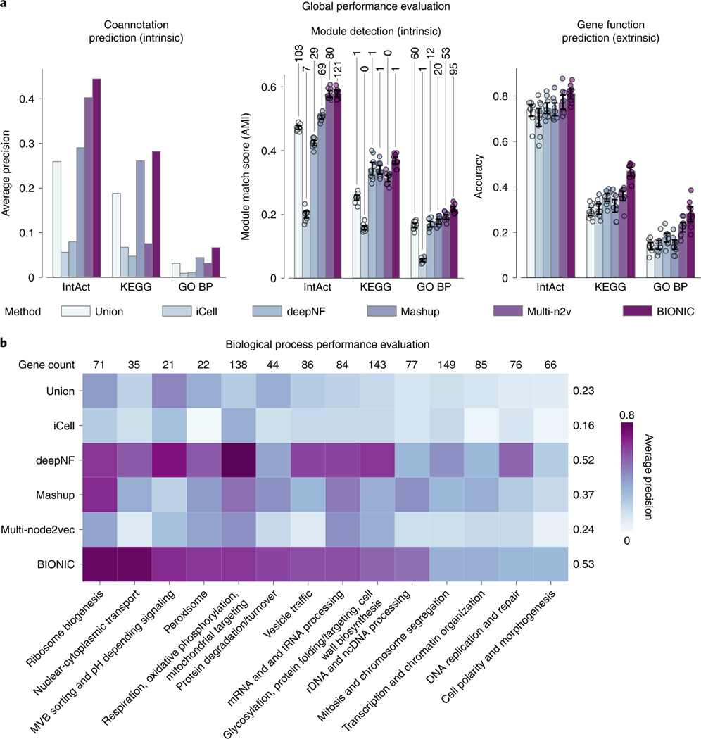
a, Coannotation prediction, module detection and gene function prediction evaluations for three yeast networks integrated by the tested unsupervised network integration methods. The input networks and evaluation standards are the same as in Fig. 2. Data are presented as mean values. Error bars indicate the 95% confidence interval for
Evaluation of BIONIC in a semisupervised setting
We also tested how BIONIC performs in a semisupervised setting (Fig. 4). Here, we compared BIONIC trained with no labeled data (unsupervised), BIONIC trained with a held-out set of functional labels given by IntAct, KEGG and GO (semisupervised), and a supervised integration algorithm using the same labels (GeneMANIA5). For each of these methods, we integrated the yeast protein–protein interaction, coexpression and genetic interaction networks from the Fig. 2 analysis. In each benchmark, 20% of genes (IntAct, KEGG, GO) were randomly held out and used as a test set, while the remaining 80% of genes were used for training. The unsupervised BIONIC did not use any gene label information for training, but it was evaluated using the same test set as the supervised methods to ensure a consistent performance comparison. To control for variability in the train-test set partitioning, this procedure was repeated ten times and the average performance across test sets was reported (Methods). We found that adding labeled data can substantially improve the features BIONIC learns and these features also outperform the integration results produced by the supervised GeneMANIA method. We also found that even without labeled data, BIONIC performs as well as, or exceeds, GeneMANIA performance. Notably, the performance of the unsupervised and semisupervised BIONIC is similar for gene function prediction. This indicates unsupervised BIONIC features are already sufficiently discriminative for classifiers to perform well. Thus, BIONIC can be used effectively in both an unsupervised and semisupervised setting, which demonstrates its versatility as a biological network integration algorithm. We also analyzed the performance of BIONIC in a scenario where labels are noisy (Supplementary Note 3 and Extended Data Fig. 8).
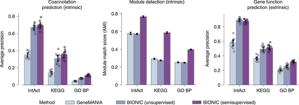
Performance comparison between a supervised network integration algorithm trained with labeled data (GeneMANIA), BIONIC trained without any labeled data (unsupervised) and BIONIC trained with labeled data (semisupervised). Bars indicate the average performance over ten trials of random train-test splits for the given benchmark (Methods). Data are presented as mean values. Error bars indicate the 95% confidence interval.
Scalability of BIONIC and established integration approaches
An effective integration algorithm should be able to scale to many network inputs and networks with many nodes. To test network input scalability, we randomly sampled progressively larger sets of yeast gene coexpression networks (Fig. 5a and Supplementary Data File 2) and assessed the performance of the resulting integrations of these sets. We similarly tested node scalability by randomly subsampling progressively larger gene sets of four human protein–protein interaction networks34–37 (Fig. 5b and Supplementary Data File 2). BIONIC can integrate numerous networks (Fig. 5a), and networks with many nodes (Fig. 5b), outperforming all other methods assessed for progressively more and larger networks. To achieve this scalability, BIONIC takes advantage of the versatile nature of deep learning technology by learning features for small batches of genes and networks at a time, reducing the computational resources required for any specific training step. To learn gene features over large networks, BIONIC learns features for random subsets of genes at each training step and randomly subsamples the local neighborhoods of these genes to perform the graph convolution (Methods), maintaining a small overall computational footprint. This subsampling allows BIONIC to integrate networks with many genes, whereas methods such as Mashup can only do so with an approximate algorithm that reduces integration performance (Supplementary Fig. 1). To integrate many networks, BIONIC uses a network-wise sampling approach, where a random subset of networks is integrated at a time during each training step. This reduces the number of parameter updates required at once, since only GCNs corresponding to the subsampled networks are updated in a given training step. We also tested the extent of BIONIC scalability in terms of computational resources (Supplementary Note 4 and Extended Data Fig. 9).
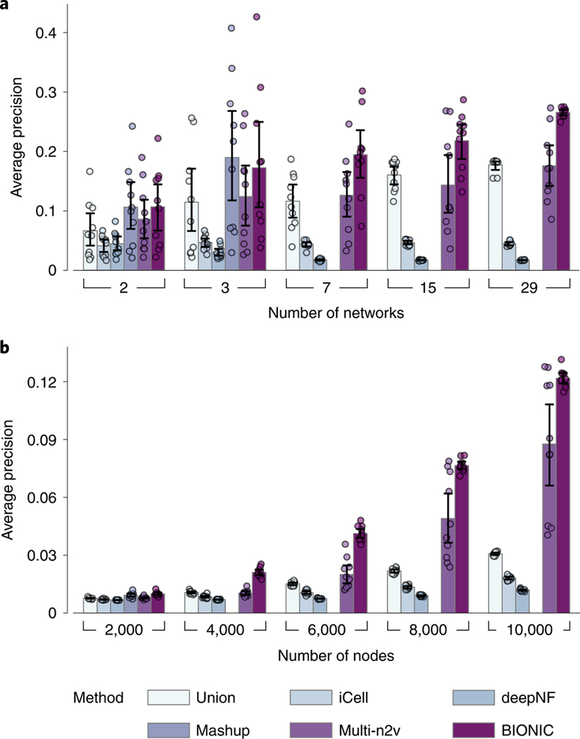
a, Performance comparison of unsupervised integration methods across different numbers of randomly sampled yeast coexpression input networks on KEGG pathways gene coannotations. b, Performance comparison of unsupervised integration methods across four human protein–protein interaction networks for a range of subsampled nodes (genes) on CORUM complexes protein coannotations. In these experiments, the Mashup method failed to scale to seven or more networks (a) and 4,000 or more nodes (b), as indicated by the absence of bars in those cases (Methods). Data are presented as mean values. Error bars indicate the 95% confidence interval for
BIONIC predictions of chemical–genetic interactions
We asked whether BIONIC can generate new, testable biological hypotheses. Chemical–genetic approaches analyze the effects of mutations on cell growth in response to compound treatment and can be used to systematically predict the molecular targets of uncharacterized compounds38. For example, if a conditional temperature sensitive (TS) mutant carries a mutation that compromises the activity of a compound’s target gene, it is often specifically hypersensitive to the compound39,40.
Previously, we generated a dataset of chemical–genetic screens, consisting of a pool of deletion mutants of 289 nonessential genes (diagnostic pool) and 1,522 compounds18. Using this data, we used BIONIC to predict chemical sensitivities for a wider set of 873 essential genes across a subset of 50 compounds. For the compound selection procedure, we used the unsupervised BIONIC integrated protein–protein interaction network, coexpression network and genetic interaction network features from the Fig. 2 analysis which we refer to as the physical, expression, and genetic (PEG) features. We selected compounds to study by identifying those that BIONIC predicts well within the diagnostic pool data. We did this by partitioning sensitive genes from each compound into train and test sets, and we used the BIONIC features to predict the test set genes using the training genes as input (Methods). The top 50 compounds, for which sensitive genes were most successfully predicted, were selected for further analysis. Sensitive essential gene predictions for each of the 50 chosen compounds were generated in a similar way to the compound selection procedure, with predictions being made on yeast essential genes rather than the diagnostic pool genes (Methods).
The BIONIC essential gene sensitivity predictions were experimentally validated using profiles for the compound set from a chemical– genetic screen using a collection of TS yeast mutants (Supplementary Data File 6). A DNA barcoded collection of 1,181 mutants containing TS alleles spanning 873 genes was constructed in a yeast genetic background that conferred drug hypersensitivity (
Out of 156 essential genes experimentally identified as sensitive to the set of 50 screened compounds, BIONIC successfully predicted 35. BIONIC significantly predicts sensitive genes for 13 out of 50 compounds under an ordered Fisher’s exact test. We also assessed more broadly whether BIONIC can correctly predict the biological process a given compound’s sensitive genes are annotated to. BIONIC sensitive gene predictions were statistically enriched (Fisher’s exact test) for 27 out of 62 annotated biological processes across compounds (Fig. 6a). We compared the quality of BIONIC’s predictions to a random baseline (Fig. 6b). Here, we generated 1,000 random permutations of the BIONIC PEG feature gene labels and computed sensitive essential gene predictions for the 50 screened compounds, as described previously. We found BIONIC sensitive gene and bioprocess predictions were substantially more accurate than the random permutations, indicating the BIONIC PEG features encode relevant information for the prediction of chemical–genetic interactions. We looked at the 13 significantly predicted compounds in more detail to see which sensitive gene predictions BIONIC correctly predicted and the corresponding ranks of those genes in the prediction list (Fig. 6c). We observed that for eight out of 13 compounds, the correct BIONIC predictions rank in the top ten most sensitive interactions. BIONIC predictions and experimental results for the 50 selected compounds can be found in Supplementary Data File 7.
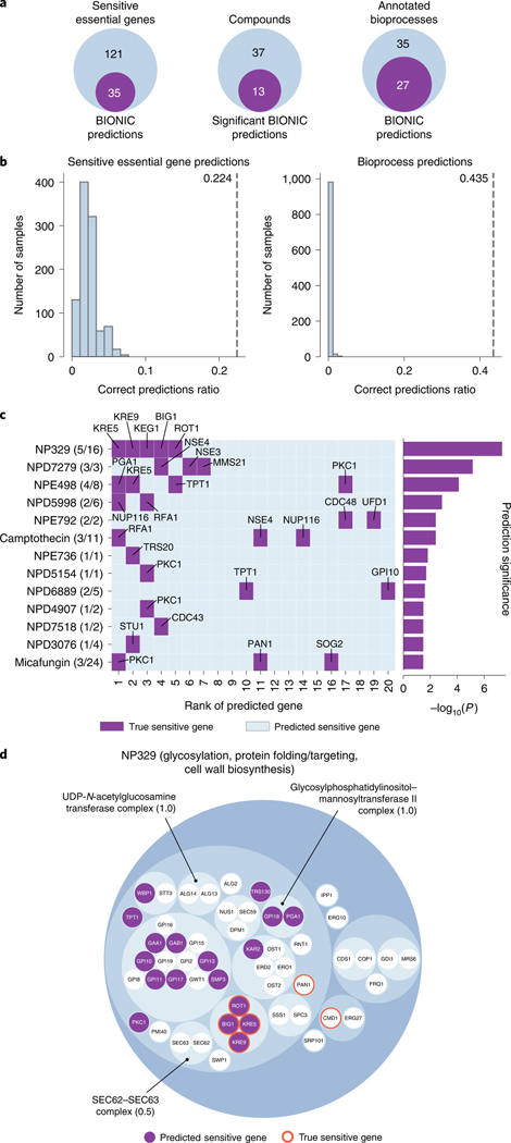
a, From left to right, the number of correct unsupervised BIONIC sensitive essential gene predictions across the 50 screened compounds, the number of compounds BIONIC significantly predicted sensitive essential genes for (ordered Fisher’s exact test) and the number of correctly predicted sensitive essential gene annotated bioprocesses, based on the bioprocess enrichment of BIONIC predictions for each compound. b, A comparison of correctly predicted sensitive genes (left) and correctly predicted biological process annotations (right) between BIONIC predictions (dashed line) and
We examined the best predicted compound, NP329, in more detail. NP329 is a pseudojervine from the RIKEN Natural Product Depository42, and among its top ten most sensitive interactions with the diagnostic pool mutants were the FLC2, DFG5, GAS1 and HOC1 (ref. 18) genes. The FCL2 product is a putative calcium channel involved in cell wall maintenance43, DFG5 encodes a glycosylphosphatidylinositol (GPI)-anchored membrane protein required for cell wall biogenesis in bud formation44, GAS1 encodes a
To further study this compound–process interaction, we hierarchically clustered the BIONIC PEG features and we focused on the essential genes present in the Fig. 2b ‘glycosylation, protein folding/targeting, cell wall biosynthesis’ bioprocess (Fig. 6d). We observed that six out of 16 NP329 sensitive essential genes lie in the bioprocess, as do 18 out of 20 BIONIC predicted sensitive essential genes. Within this bioprocess, BIONIC successfully predicts four (BIG1, KRE5, KRE9, ROT1) out of the six NP329 sensitive essential genes. These results indicate that BIONIC is able to both predict a relevant biological process targeted by the compound and the specific sensitive genes. Moreover, the four sensitive genes successfully predicted by BIONIC were all closely clustered together based on the integrated BIONIC features (Fig. 6). ROT1 encodes an essential chaperone required for N- and O-glycosylation in yeast50 and is required for normal levels of
Discussion
BIONIC is a deep learning algorithm that extends the GCN architecture to integrate biological networks. BIONIC produces gene features that capture functional information well when compared to other unsupervised methods12,17 as determined by a range of benchmarks and evaluation criteria. BIONIC can use labeled data in a semisupervised fashion when it is available, and it can be purely unsupervised otherwise. BIONIC scales to a greater number of input networks and network sizes compared to established unsupervised methods.
BIONIC can be used to predict pairs of related genes (coannotation prediction), identify functional gene modules (module detection) and accurately predict functional gene labels (gene function prediction). One of the main goals of this work is to generate fully integrated features encoding functional information for a particular organism, such that the resulting features can be used to predict numerous different aspects of cell and organism function56. As a proof-of-concept, we integrated three different yeast networks, incorporating protein–protein interaction, coexpression and genetic interaction data. We also used BIONIC features to generate predictions for essential gene chemical sensitivities and a substantial number were experimentally validated, indicating BIONIC is effective at prediction and hypothesis generation.
BIONIC is capable of capturing relevant functional information across input networks. However, input networks do not have uniform quality and some networks may only describe certain types of functional relationship effectively (such as those within a particular biological process) while obscuring other relationships. Indeed, while BIONIC is able to capture a greater number of functional modules in an integrated network compared to a single input network (Fig. 2c and Extended Data Fig. 5), it does not capture every functional module present in the input networks (Fig. 2c, Extended Data Fig. 5 and Supplementary Data Files 4 and 5). This is likely due to some networks obscuring signals present in other networks. Implementing more advanced input network feature weighting should ensure that high-quality information is preferentially encoded in the learned features and that low-quality information is not. This may help to identify which functional relationships are driven by which networks and network types, thereby indicating which parts of the functional range have good or poor coverage and identifying areas to target for future experimental work.
The naive union of networks approach performs well, motivating its inclusion as a baseline in any network integration algorithm assessment. While the union network contains all possible relationships across networks, it likely contains relatively more false-positive relationships in the integrated result, since all false-positives in the input networks are retained by the union operation. Thus, the union should work well for high-quality networks, but perform poorly with noisy networks.
Our chemical–genetic analysis demonstrates the potential of BIONIC to provide target predictions from limited experimental data. While BIONIC performs well at predicting essential gene chemical– genetic interactions, further improvements in performance could potentially be made through an optimized choice of input networks that specifically indicate these chemical sensitivities. BIONIC chemical–genetic interaction predictions could also be used to instead generate a set of putative nonsensitive genes for a given compound, indicating bioprocesses where the compound is not active. This would reduce the size of the experimental space when screening, resulting in more rapid and less expensive data generation. Finally, strong BIONIC chemical–genetic interaction predictions that are not reflected in the experimental data could indicate experimental false negatives that require additional investigation.
BIONIC learns gene features based solely on their topological role in the given networks. A powerful future addition to BIONIC would be to include gene or protein features such as amino acid sequence57, protein localization58, mutant morphological defect59 or other nonnetwork features to provide additional context for genes in addition to their topological role. Continued development of integrative gene function prediction using deep learning-based GCN and encoder–decoder technologies will enable us to map gene function more richly and at larger scales than previously possible.
Online content
Any methods, additional references, Nature Research reporting summaries, source data, extended data, supplementary information, acknowledgements, peer review information; details of author contributions and competing interests; and statements of data and code availability are available at https://doi.org/10.1038/s41592-022-01616-x.
Methods
BIONIC method overview
An undirected input network can be represented by its adjacency matrix
BIONIC encodes each input network using instances of a GCN variant known as the graph attention network (GAT)17. We selected this architecture because of its considerable performance improvements over existing architectures on a range of node classification tasks17. The GAT has the ability to learn alternative network edge weights, allowing it to downweight or upweight edges based on their importance for the network reconstruction task. In the original formulation, the GAT assumes binary network inputs. We modify the GAT to consider a priori network edge weights. The GAT formulation is then given by:
where
Here,
where
Initial node features
Here,
The mask
We found that learning the integrated features in this joint manner (learning and combining network-specific features end-to-end) performs better than simply concatenating the network-specific features (that is, late fusion), indicating that BIONIC is able to learn complementary information across input networks (Supplementary Fig. 3).
To obtain the final, integrated node features
To obtain a high-quality
The unsupervised loss is then given by:
where
For the semisupervised training objective, BIONIC first predicts gene labels by mapping
where
where
The final loss BIONIC trains to minimize is a weighted sum of the unsupervised and semisupervised losses:
where
Implementation details
BIONIC was implemented using PyTorch60, a popular Python-based deep learning framework, and relies on functions and classes from the PyTorch Geometric library61. It uses the Adam62 optimizer to train and update its weights. To be scalable in the number of networks, BIONIC uses an optional network batching approach where subsets of networks are sampled and integrated at each training step. The sampling procedure is designed so that each network is integrated exactly once per training step. Network batching yields a constant memory footprint at the expense of increased runtime with no empirical degradation of feature quality. This feature is provided for additional scalability over what is demonstrated in this work and was not used in any of our reported experiments. Additionally, BIONIC is scalable in the number of network nodes. It uses a node sampling approach (equivalent to mini-batch training, where nodes are samples) to learn features for subsets of nodes in a network, and a neighborhood sampling procedure to subsample node neighborhoods. Node sampling ensures only part of a network needs to be retained in memory at a time while neighborhood sampling reduces the effective higher-order neighborhood size in sequential GAT passes, again reducing the number of nodes required to be retained in memory at any given time, further reducing BIONIC’s memory footprint.
For very large networks where the initial node feature matrix (that is, the identity matrix) cannot fit into memory due to limitations with PyTorch matrix operations, BIONIC incorporates a singular value decomposition-based approximation. First, the union of networks is computed by creating a network that contains the nodes and edges of all input networks. If an edge occurs in multiple networks, the maximum weight is used. A low-dimensional singular value decomposition approximation of the normalized Laplacian matrix of the union network is computed and used as the initial node features for each network. Finally, BIONIC uses sparse representations of network adjacency matrices (except for the input node feature matrix, see above), further reducing memory footprint. All BIONIC integration experiments in this paper were run on an NVIDIA Titan Xp graphical processing unit with 12 GB of video RAM, no more than 16 GB of system RAM and a single 2.4 GHz Intel Xeon CPU.
Network preprocessing
The yeast protein–protein interaction network20 and human protein–protein interaction networks34–37 were obtained from BioGRID63, genetic interaction profiles22 were obtained directly from the published supplementary data of Costanzo et al.22, and gene expression profiles21 were obtained from the SPELL database64. These networks were chosen since they had the most functional information compared to other networks in their class (that is, protein–protein interaction networks, coexpression networks and genetic interaction networks). To create a network from the genetic interaction profiles, genes with multiple alleles were collapsed into a single profile by taking the maximum profile values across allele profiles. Pairwise Pearson correlation between the profiles was then calculated, and gene pairs with a correlation magnitude greater than or equal to 0.2 were retained as edges, as established22. For the gene expression profiles, networks were constructed by retaining gene pairs with a profile Pearson correlation magnitude in the 99.5th percentile. Coexpression and genetic interaction networks had their edge weights normalized to the range [0, 1].
Obtaining integrated results
The naive union of networks benchmark was created by taking the union of node sets and edge sets across input networks. For edges common to more than one network, the maximum weight was used. For all other methods, automated hyperparameter optimization was performed to ensure hyperparameters were chosen consistently and fairly. Here, a S. pombe genetic interaction network27, coexpression network26 and protein–protein interaction network25 were used as inputs to the integration methods. To perform one iteration of the hyperparameter optimization, a random combination of hyperparameters was uniformly sampled over a range of reasonable values for each method and used to integrate the three pombe networks. The integration results were then evaluated using a pombe protein complex standard (obtained from https://www.pombase.org/data/annotations/Gene_ontology/GO_complexes/Complex_annotation.tsv). The evaluations consisted of a coannotation prediction, module detection and gene function prediction assessment (Evaluation methods). This procedure was repeated for 50 combinations of hyperparameters, for each method. For methods that produced features (deepNF, Mashup, multi-node2vec and BIONIC), a feature dimension of 512 was used to ensure results were comparable across methods. For methods that required a batch size parameter (deepNF and BIONIC), the batch size was set to 2,048 to ensure reasonable computation times. Hyperparameter combinations were then ranked for each method across the three evaluation types and the hyperparameter combination corresponding to the highest average rank across evaluation types was chosen. The hyperparameter optimization results are found in Supplementary Data File 1. Note that the union method was not included in the hyperparameter optimization because it has no hyperparameters. Additionally, the Mashup method used 44 hyperparameter combinations rather than 50, as six hyperparameter combinations exhausted the available memory resources and did not complete.
All integration results reported were obtained by integrating networks using the set of hyperparameters identified in the hyperparameter optimization procedure. BIONIC features used in the Figs. 2, ,33 and and66 analyses are found in Supplementary Data File 8. Coannotation prediction, module detection and gene function prediction standards used in Figs. 2–5 are found in Supplementary Data File 9.
Benchmark construction
Functional benchmarks were derived from GO Biological Process ontology annotations, KEGG pathways and IntAct complexes for yeast, and CORUM complexes for human (Supplementary Data File 3). Analyses were performed using positive and negative gene pairs, clusters or functional labels obtained from the standards as follows: the GO Biological Process benchmark was produced by filtering Inferred from Electronic Annotation (IEA) annotations, as they are known to be lower quality, removing genes with dubious open reading frames and filtering terms with more than 30 annotations (to prevent large terms, such as those related to ribosome biogenesis, from dominating the analysis65). We found the performance evaluations to be robust to this threshold (Supplementary Fig. 6). For the coannotation benchmark, all gene pairs sharing at least one annotation were retained as positive pairs, while all gene pairs not sharing an annotation were considered to be negative pairs. KEGG, IntAct and CORUM benchmarks were produced analogously, without size filtering.
For the module detection benchmark, clusters were defined as the set of genes annotated to a particular term, for each standard. Modules of size 1 (singletons) were removed from the resulting module sets as they are uninformative. For the per-module analyses in Fig. 2c, Extended Data Figs. 4 and and55 and Supplementary Data Files 4 and 5, we also removed any modules of size 2 since these modules had highly variable Jaccard scores.
The supervised standards were obtained by treating each gene annotation as a class label, leading to genes with multiple functional classes (that is, a multi-label classification problem). The standards were filtered to only include classes with 20 or more members for GO Biological Process and KEGG, or ten members for IntAct. This was done to remove classes with very few data points, ensuring more robust evaluations.
The granular function standard in Figs. 2b, ,3b3b and and66 was obtained from the Costanzo et al.22 supplementary materials. Any functional category with fewer than 20 gene members was removed from the analysis to ensure only categories with robust evaluations were reported.
Evaluation methods
We used a precision-recall-based coannotation framework to evaluate individual networks and integrated results. We used precision-recall instead of receiving operator curve because of the substantial imbalance of positives and negatives in the pairwise benchmarks for which the receiving operator curve would overestimate performance. Here, we computed the pairwise cosine similarities between gene profiles in each network or integration result. Due to the high-dimensionality of the datasets, cosine similarity is a more appropriate measure than Euclidean distance since the contrast between data points is reduced in high-dimensional spaces under Euclidean distance66. Precision-recall operator points were computed by varying a similarity threshold, above which gene or protein pairs are considered positives and below which pairs are considered negative. Each set of positive and negative pairs was compared to the given benchmark to compute precision and recall values. To summarize the precision-recall curve into a single metric, we computed average precision (AP) given by:
where
The module detection evaluation was performed by clustering the integrated results from each method and comparing the coherency of resulting clusters with the module-based benchmarks. Since the benchmarks contain overlapping modules (that is, one gene can be present in more than one module) that prevent the use of many common clustering evaluation metrics (since these metrics assume unique assignment of gene to cluster), the module sets are subsampled during the evaluation to ensure there are no overlapping modules (the original module sets are used as-is for the per-module-optimized experiments in Extended Data Fig. 5 and Supplementary Data File 5). Next, the integrated results are hierarchically clustered with a range of distance metrics (Euclidean and cosine), linkage methods (single, average and complete) and thresholds to optimize benchmark comparisons over these clustering parameters (this is done for all methods that are compared). The resulting benchmark-optimized cluster sets are compared to the benchmark module sets by computing adjusted mutual information: an information theoretic comparison measure that is adjusted to normalize against the expected score from random clustering. The highest adjusted mutual information score for each integration approach is reported, ensuring the optimal cluster set for each dataset across clustering parameters is used for the comparison and that our results are not dependent on clustering parameters. Finally, this procedure is repeated ten times to control for differences in scores due to the cluster sampling procedure. The sets of clustering parameter-optimized BIONIC clusters obtained from the Fig. 2 integration for each standard are in Supplementary Data File 4.
To perform the supervised gene function prediction evaluation, ten trials of five-fold cross validation were performed using SVM classifiers each using a radial basis function kernel24. The classifiers were trained on a set of gene features obtained from the given integration method with corresponding labels given by the IntAct, KEGG and GO Biological Process supervised benchmarks in a one-versus-all fashion (since each individual gene has multiple labels). Each classifier’s regularization and gamma parameters were tuned in the validation step. For each trial, the classifier results were evaluated on a randomized held-out set consisting of 10% of the gene features not seen during training or validation and the resulting classification accuracy was reported. We repeated this entire procedure for a random forest68 and a gradient boosted trees69 classifier and found BIONIC also outperforms the compared integration methods, indicating the SVM classifier is not biased toward improving BIONIC performance (Supplementary Fig. 7).
The granular functional evaluations in Figs. 2b and and3b3b were generated by computing the average precision (as mentioned in the precision-recall evaluation framework description) for the gene subsets annotated to the given functional categories.
To perform the module comparison analysis in Fig. 2c, we additionally applied the module detection analysis performed in Fig. 2a to the input networks. Here, the interaction profiles of the networks were treated as gene features and the clustering parameters were optimized to best match the IntAct complexes standard. We compared the resulting module sets from the input networks and BIONIC features to known protein complexes given by the IntAct standard. For each complex in the standard, we reported the best-matching predicted module in each dataset as determined by the overlap (Jaccard) score between the module and the known complex (Supplementary Data File 4). To generate the Venn diagram, we defined a complex to have been captured in the dataset if it had an overlap score of 0.5 or greater with a predicted module.
To perform the LSM2–7 module analysis in Fig. 2d, we analyzed the predicted module in each dataset that had the highest overlap score with the LSM2–7 complex. We created a network from the BIONIC features by computing the cosine similarity between all pairs of genes and setting all similarities below 0.5 to zero. The resulting nonzero values were then treated as weighted edges to form a network. We extracted a subnetwork from each of the protein–protein interaction, coexpression, genetic interaction and newly created BIONIC networks, consisting of the best scoring predicted module and the genes showing direct interactions with those in the predicted module. We laid out these networks using the spring-embedded layout algorithm in Cytoscape70. The edges in the protein–protein interaction network correspond to direct, physical interactions, and the edges in the coexpression and genetic interaction networks correspond to the pairwise Pearson correlation of the gene profiles, as described above.
To perform the semisupervised network integration experiment in Fig. 4, we first generated randomized train and test sets. Here, 20% of genes were randomly held out in each gene function benchmark (IntAct, KEGG and GO Biological Process) separately and retained for downstream evaluations. These benchmarks consist of functional labels for a set of yeast genes (protein complex membership in IntAct, pathway membership in KEGG and biological process annotation in GO Biological Process) and are the same benchmarks used in the gene function prediction evaluation (Figs. 2a and and3a).3a). The remaining 80% of genes were used for training GeneMANIA and BIONIC. To generate test sets for the coannotation prediction benchmarks, we removed any coannotations where both genes were present in the training set. To generate test sets for the module detection benchmarks, we removed any modules consisting entirely of genes in the training set. We then integrated the three yeast networks from the Figs. 2 and and33 analysis (a protein–protein interaction20, gene coexpression21 and genetic interaction network22) using the supervised GeneMANIA, BIONIC without using any labeled data (unsupervised) and a semisupervised mode of BIONIC that uses the labeled data (semisupervised). Each integration result was then evaluated using the held-out test data. For the coannotation prediction and module detection evaluations, the integrated features from BIONIC (both unsupervised and semisupervised) and the integrated network from GeneMANIA were evaluated. Both GeneMANIA and the semisupervised BIONIC generate gene label predictions directly, without the need for an additional classifier such as in the Fig. 2a gene function prediction evaluation. However, the unsupervised BIONIC does not generate gene label predictions (since it is given no labeled information to begin with). To ensure a consistent comparison with GeneMANIA and the semisupervised BIONIC, we trained a classification head on top of the unsupervised BIONIC. The classification head architecture is identical to the semisupervised BIONIC classification head, however, in the unsupervised case we only allow gradients from the classification loss objective to backpropagate to the classification head, not the rest of the model. This ensures a comparable classification model can be trained on top of the unsupervised BIONIC model, without the labeled data affecting the model weights such as in the semisupervised case. GeneMANIA does not generate multi-label predictions, and so we used GeneMANIA to generate label predictions for each class individually and then performed Platt scaling to convert these binary class predictions to multi-label predictions7,71. The gene function prediction evaluations were then performed by comparing the gene label predictions from the integration methods, to the held-out test labels. This entire procedure, starting with the train-test set partitioning, to the final evaluations, was repeated a total of ten times to control for performance variability due to the partitioning procedure.
Network scaling experiment
To perform the network scaling experiment, we uniformly sampled subsets of the yeast coexpression networks (Supplementary Data File 2). We performed ten integration trials for each network quantity, and these trials were paired (that is, each method integrated the same randomly sampled sets of networks). The average precision scores of the resulting integrations with respect to the KEGG pathways coannotation standard (Supplementary Data Files 3) were then reported. The Mashup method did not scale to the seven-network input size or beyond on a machine with 64 GB of RAM.
Node scaling experiment
The node scaling experiment was performed by uniformly subsampling the nodes of four large human protein–protein interaction networks34–37 (Supplementary Data File 2) for a range of node quantities and integrating these subsampled networks. Ten trials of subsampling were performed for each number of nodes (paired, as above) and the average precision scores with respect to the CORUM complexes coannotation standard (Supplementary Data File 3) were reported. The Mashup method did not scale to 4,000 nodes or beyond on a machine with 64 GB of RAM.
Gene chemical sensitivity predictions
Chemical–genetic profiles against a diagnostic set of 310 nonessential yeast gene deletion mutants were obtained from a previous study18. The genes were chosen using the COMPRESS-GI algorithm, which selected a set of 157 genes capturing most of the functional information within genome-wide genetic interaction data72, along with 153 genes that were manually selected to complement the set. Haploid deletion mutants for the gene set were constructed in a genetic background that conferred drug hypersensitivity (
Here,
To predict chemical–genetic interactions using BIONIC, we first selected a set of 50 compounds to generate predictions on and experimentally validate. For each diagnostic pool compound, we filtered out any genes not present in the integrated BIONIC features (the same features used for the Figs. 2 and and33 analyses, referred to as PEG features). Any compounds with fewer than two outlier sensitive genes were then removed. For each of the remaining compounds, we randomly split the sensitive genes into train and test sets. Next, for a given compound, we computed BIONIC predictions for the test set genes. We did this by averaging the corresponding BIONIC PEG features for each gene in the training set under a cosine distance metric to get a representative feature vector in gene feature space for the given compound. The BIONIC predictions for the compound were then obtained by identifying the top 20 nearest genes to this feature vector (excluding genes in the training set).
To obtain a score for the BIONIC predictions, an ordered Fisher’s exact test was performed between the test set genes and the BIONIC predictions as follows:
where
The above process was repeated five times for new randomly sampled train and test gene splits, or up to the maximum number of train-test splits possible for compounds with fewer than five sensitive genes. Final
The BIONIC gene chemical sensitivity predictions were benchmarked against experimental data obtained from chemical–genetic screens using a collection of TS mutants for essential genes. We previously constructed a drug-hypersensitive, barcoded set of TS mutants for 1,181 TS alleles spanning 837 essential genes40. Similar to the diagnostic set of nonessential genes, this collection also contained the
The significance of BIONIC sensitive essential gene predictions for each compound was determined by using an ordered Fisher’s exact test, as detailed above. The Benjamini–Hochberg procedure74 was applied to the resulting
To generate biological process22 predictions as reported in Fig. 6a,,b,b, a Fisher’s exact test was performed between the full set of 20 BIONIC gene predictions and biological process gene annotations. We used the same annotations as in Figs. 2b and and3b3b (ref. 22). If the BIONIC sensitive gene predictions were enriched for one or more bioprocesses, and these bioprocesses overlapped with the annotated bioprocess of the true sensitive genes, we considered this a correct bioprocess prediction. To generate the random benchmark in Fig. 6b, the gene labels of the BIONIC integrated features were randomly permuted and new essential sensitive gene predictions for the 50 selected compounds were generated in the same manner as the original BIONIC predictions (detailed above). This process was repeated for 1,000 random gene label permutations to generate the benchmark distributions. The circle plot in Fig. 6d was produced by first hierarchically clustering the integrated BIONIC gene features, subsetted to essential genes annotated to the glycosylation, protein folding/targeting, cell wall biosynthesis bioprocess. Two clustering thresholds were chosen to generate clusters, broadly indicating the hierarchical organization of the BIONIC gene features. The first, most granular clustering threshold was adaptively chosen to generate clusters best-matching known protein complexes, as defined by the IntAct complexes standard29. For each protein complex in the standard, the clustering threshold was optimized to produce the cluster best matching this protein complex. For clusters not matching known complexes, the largest complex optimized threshold was used. The second, higher clustering threshold was set to a cophenetic distance of 0.9.
The BIONIC essential gene sensitivity predictions can be found in Supplementary Data File 7.
Quantification of
Wild-type (
Reporting summary
Further information on research design is available in the Nature Research Reporting Summary linked to this article.
Extended Data
Extended Data Fig. 1 |

A more detailed view of an individual network encoder, including residual connections. A network specific graph convolutional network is used to encode the input network for increasing neighborhood sizes. The first GCN in the sequence learns features for a given node based on the node’s immediate neighborhood (1st order features). The next GCN learns features based on the node’s second order neighborhood (2nd order features), and so on. The node feature matrices learned by each GCN pass are summed together to create the final learned, network-specific features. Summing the outputs of the various GCNs in this way creates residual connections, allowing features from multiple neighborhood sizes to generate the final learned features, rather than just the final neighborhood size. This figure shows three GCN layers, but BIONIC uses the same pattern of connections for any number of GCN layers. Note that the GCN layers for a given encoder share their weights, so in effect, there is a single GCN layer for each encoder.
Extended Data Fig. 2 |
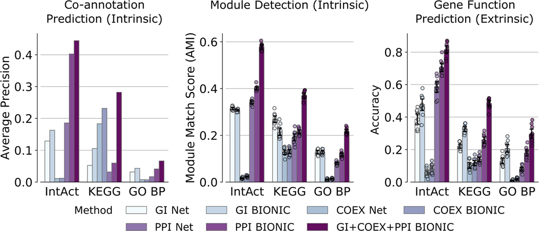
A comparison of individual networks (denoted ‘Net’), their corresponding features encoded using the unsupervised BIONIC (denoted ‘BIONIC’), as well as the BIONIC integration of these networks (denoted ‘GI+COEX+PPI BIONIC’). BP = Biological Processes, GI = Genetic Interaction, COEX = Co-expression, PPI = Protein-protein Interaction. These are the same networks and evaluations used in Fig. 2. Data are presented as mean values. Error bars indicate the 95% confidence interval for n = 10 independent samples.
Extended Data Fig. 3 |
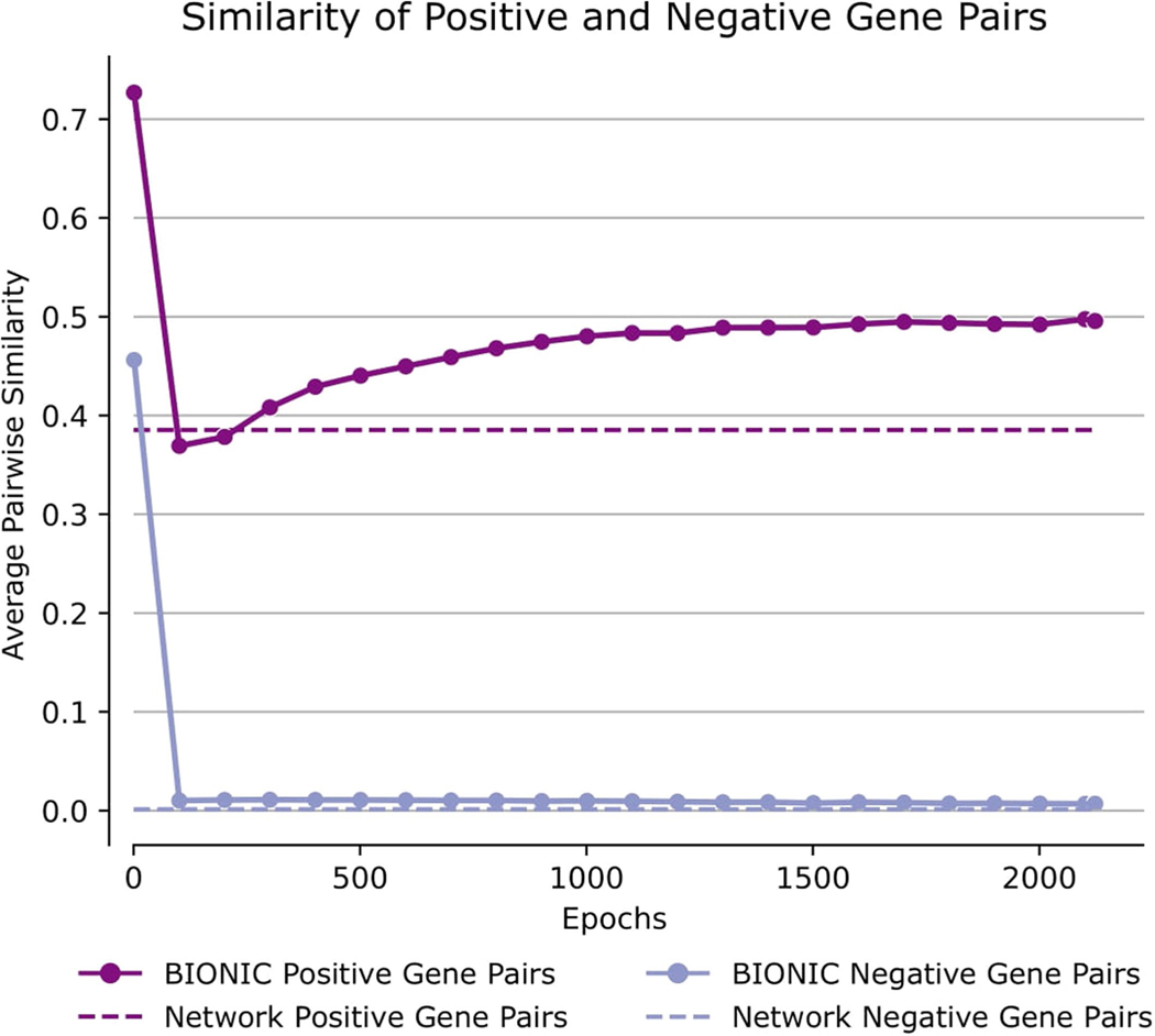
Comparison of pairwise gene similarities (cosine similarity in the case of BIONIC, direct binary adjacency in the case of the network), as defined by IntAct Complexes for known co-complex relationships (positive pairs) and no co-complex relationships (negative pairs), between a yeast PPI network (as used in the Fig. 2 analyses) and the unsupervised BIONIC features produced from this network. The BIONIC similarities are shown throughout the training process (epochs), whereas the input network is constant so its pairwise similarities do not change. ‘Network’ denotes the input PPI network, ‘BIONIC’ denotes the features learned from this network using BIONIC.
Extended Data Fig. 4 |
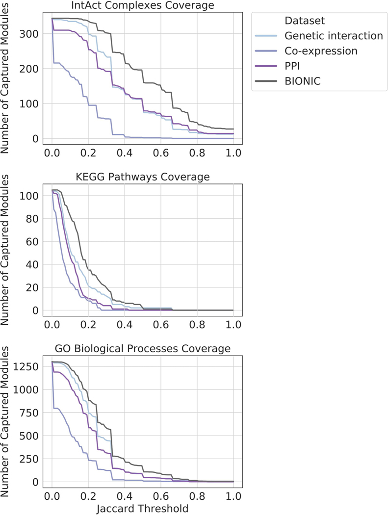
Coverage of functional gene modules by individual networks and the unsupervised BIONIC integration of these networks (denoted BIONIC), as determined by a parameter optimized module detection analysis where the clustering parameters were optimized for each module individually. The number of captured modules is reported for a range of overlap scores (Jaccard threshold). Higher threshold indicates greater correspondence between the clusters obtained from the dataset and their respective modules given by the standard. PPI = protein-protein interaction. These are the same networks and BIONIC features as Fig. 2.
Extended Data Fig. 5 |
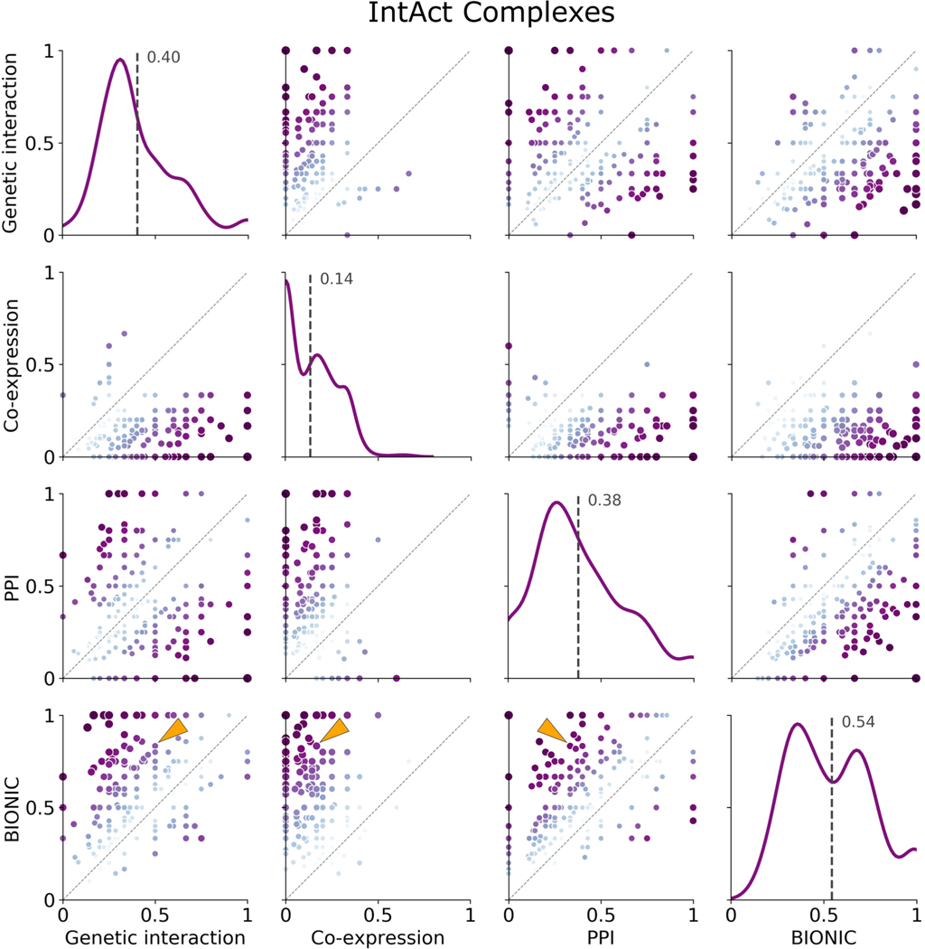
Known protein complexes (as defined by the IntAct standard) captured by individual networks and the unsupervised BIONIC integration of these networks (denoted BIONIC). Hierarchical clustering was performed on the datasets and resulting clusters were compared to known IntAct complexes and scored for set overlap using the Jaccard score (ranging from 0 to 1). The clustering algorithm parameters were optimized for each module individually, unlike the analysis in Fig. 2 where the clustering parameters were optimized for the standard as a whole. Each point is a protein complex, as in Fig. 2c. The dashed line indicates instances where the given data sets achieve the same score for a given module. Histograms indicate the distribution of overlap (Jaccard) scores for the given dataset, and the labelled dashed line indicates the mean of this distribution. The individual modules shown here as well as for the KEGG Pathways and IntAct Complexes module standards can be found in Supplementary Data File 4. The LSM2–7 complex is indicated by the arrows. PPI = protein-protein interaction. This analysis uses the same networks and BiONIC features as Fig. 2.
Extended Data Fig. 6 |
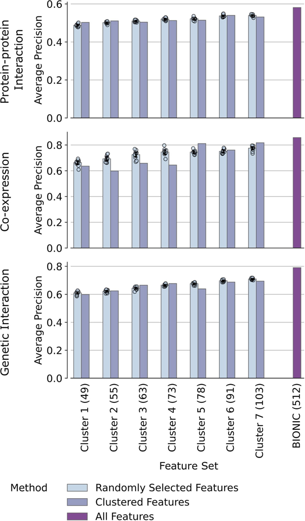
Co-annotation evaluations of the unsupervised BIONIC features subset to different clusters of feature dimensions (denoted ‘Cluster’). The number of feature dimensions for each cluster is given in parenthesis. The performance of the original BIONIC features (denoted BIONIC (512)) is also displayed. Data are presented as mean values. Bars indicate 95% confidence interval for n = 10 independent samples.
Extended Data Fig. 7 |
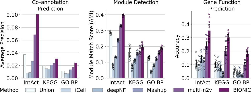
Performance comparison of 5 yeast-two-hybrid network integrations across functional standards, evaluation types and unsupervised integration methods. Data are presented as mean values. Bars indicate 95% confidence interval for n = 10 independent samples. BP = Biological Process, multi-n2v = multi-node2vec.
Extended Data Fig. 8 |
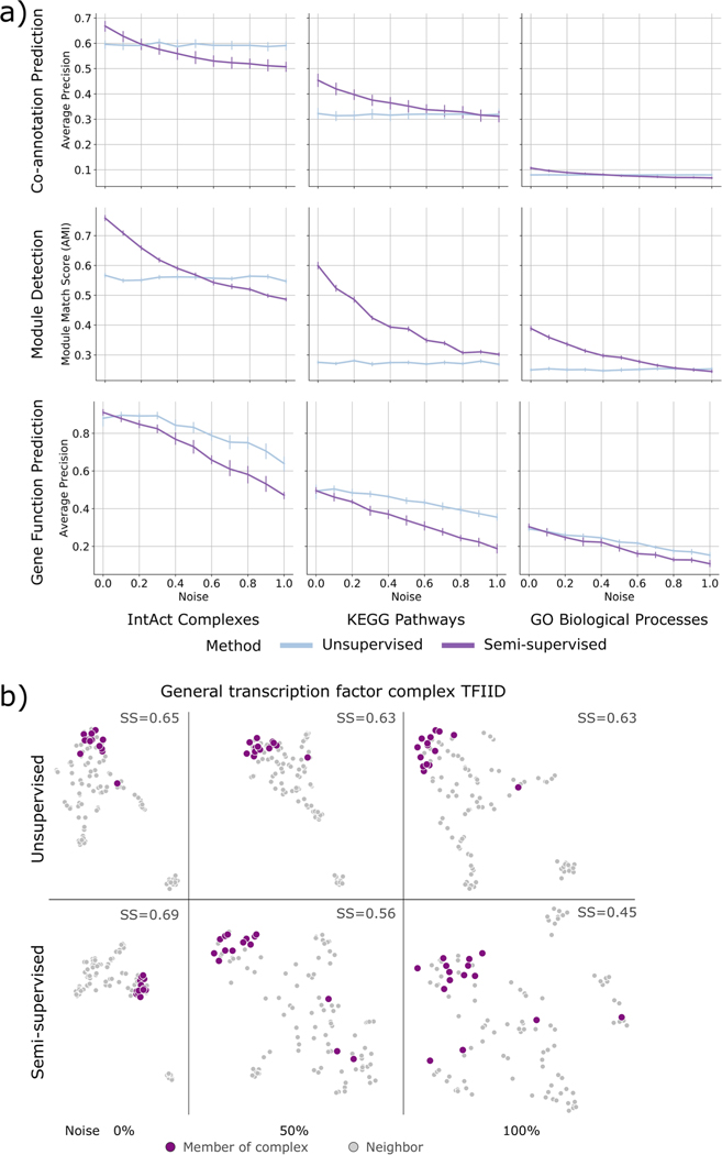
Semi-supervised BIONIC comparisons. a) A label poisoning experiment, where progressively more permutation noise is added to the label sets the semi-supervised BIONIC is trained on. ‘Noise’ indicates the proportion of permutation noise applied (multiply by 100 for percentages). Data are presented as mean values. Bars indicate 95% confidence interval for n = 10 independent samples. b) UMAP plots comparing the embedding space of the TFIID complex and the 100 nearest neighbors of this complex for unsupervised and semi-supervised BIONIC over a range of label noise values. SS = average silhouette score of TFIID members.
Extended Data Fig. 9 |
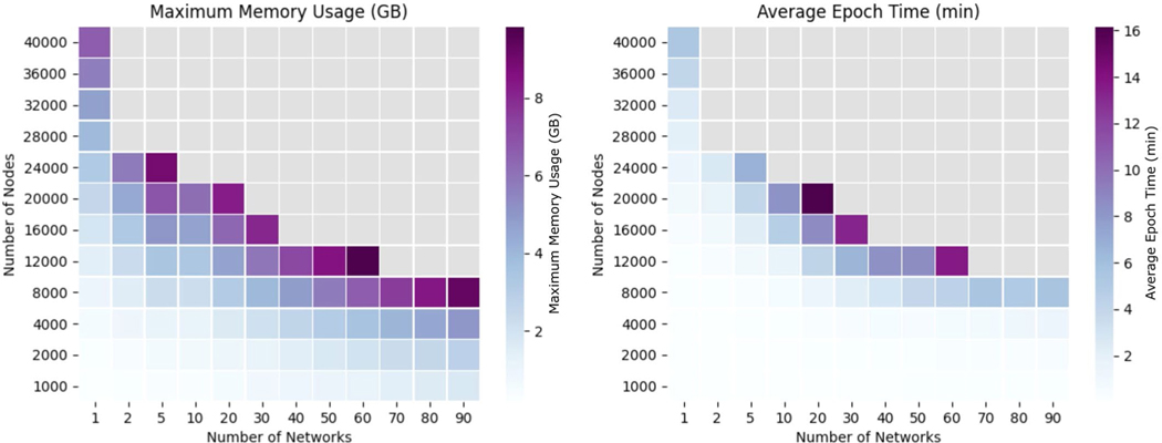
Graphics processing unit (GPU) memory usage in gigabytes (left) and average wall clock epoch time in minutes (right) for a range of network sizes and number of networks. GB = gigabyte, min = minutes. Gray squares indicate a scenario where BIONIC exceeded the maximum memory of the GPU and failed to complete. The experiments were run on a Titan Xp GPU with a 2.4 GHz Intel Xeon CPU and 32 GB of system memory.
Extended Data Fig. 10 |
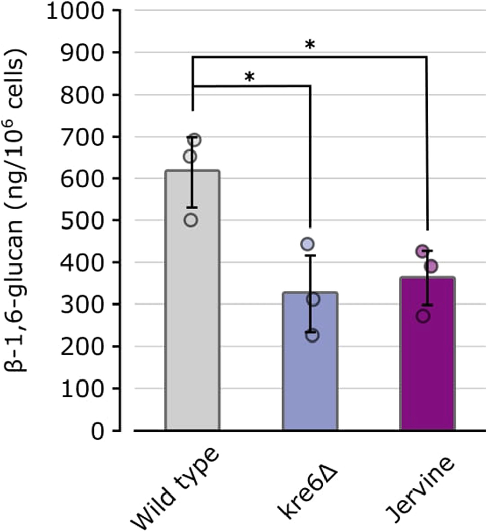
The amount of glucan per cell was calculated using pustulan as a standard. Data are presented as mean values. Error bars indicate standard deviation for n = 3 biologically independent samples.
Acknowledgements
We thank B. Andrews, M. Costanzo and C. Myers for their insightful comments. We also thank M. Fey for adding important features to the PyTorch Geometric library for us. This work was supported by NRNB (US National Institutes of Health, National Center for Research Resources grant number P41 GM103504). Funding for continued development and maintenance of Cytoscape is provided by the US National Human Genome Research Institute under award number HG009979. This work was also supported by the Canadian Institutes of Health Research Foundation grant number FDN-143264, US National Institutes of Health grant number R01HG005853 and joint funding by Genome Canada (OGI-163) and the Ministry of Economic Development, Job Creation and Trade, under the program Bioinformatics and Computational Biology. This work was supported by the National Research Council of Canada through the AI for Design program. This work was supported by CIFAR AI Chair programs. This work was also supported by JSPS KAKENHI grant numbers JP15H04483 (C.B. and Y.O.), JP17H06411 (C.B. and Y.Y.), JP18K14351 (K.I.-N.), JP19H03205 (Y.O.), JP20K07487 (D.Y.) and a RIKEN Foreign Postdoctoral Fellowship (S.C.L.). This research was enabled in part by support provided by SciNet and the Digital Research Alliance of Canada.
Footnotes
Code availability
The BIONIC code is available at https://github.com/bowang-lab/BIONIC77. Code to reproduce the main figure analyses (Figs. 2–6) is available at https://github.com/duncster94/BIONIC-analyses78 and a library implementing the coannotation prediction, module detection and gene function prediction evaluations is available at https://github.com/duncster94/BIONIC-evals 79. The BIONIC integrated yeast features (PEG features) can be explored at https://bionicviz.com.
Competing interests
The authors declare no competing interests.
Additional information
Extended data are available for this paper at https://doi.org/10.1038/s41592–022-01616-x.
Supplementary information The online version contains supplementary material available at https://doi.org/10.1038/s41592-022-01616-x.
Peer review information Nature Methods thanks Kevin Yuk-Lap Yip and the other, anonymous, reviewer(s) for their contribution to the peer review of this work. Primary Handling Editor: Lin Tang, in collaboration with the Nature Methods team.
Reprints and permissions information is available at www.nature.com/reprints.
Data availability
All data, standards, BIONIC yeast features and chemical–genetic interaction data are available in the following Figshare repository: https://figshare.com/projects/BIONIC_Biological_Network_Integration_using_Convolutions/122585. There are no restrictions on the data. Source data are provided with this paper.
References
Citations & impact
Impact metrics
Citations of article over time
Alternative metrics

Discover the attention surrounding your research
https://www.altmetric.com/details/136738142
Smart citations by scite.ai
Explore citation contexts and check if this article has been
supported or disputed.
https://scite.ai/reports/10.1038/s41592-022-01616-x
Article citations
Progress and opportunities of foundation models in bioinformatics.
Brief Bioinform, 25(6):bbae548, 01 Sep 2024
Cited by: 0 articles | PMID: 39461902 | PMCID: PMC11512649
Review Free full text in Europe PMC
Multi-modal contrastive learning of subcellular organization using DICE.
Bioinformatics, 40(suppl 2):ii105-ii110, 01 Sep 2024
Cited by: 0 articles | PMID: 39230695 | PMCID: PMC11520230
Current and future directions in network biology.
Bioinform Adv, 4(1):vbae099, 14 Aug 2024
Cited by: 1 article | PMID: 39143982 | PMCID: PMC11321866
Contextual AI models for single-cell protein biology.
Nat Methods, 21(8):1546-1557, 22 Jul 2024
Cited by: 2 articles | PMID: 39039335 | PMCID: PMC11310085
Mapping the Multiscale Proteomic Organization of Cellular and Disease Phenotypes.
Annu Rev Biomed Data Sci, 7(1):369-389, 24 Jul 2024
Cited by: 1 article | PMID: 38748859 | PMCID: PMC11343683
Review Free full text in Europe PMC
Go to all (21) article citations
Data
Data behind the article
This data has been text mined from the article, or deposited into data resources.
BioStudies: supplemental material and supporting data
Quick GO (3)
- (1 citation) GO - GO0071554
- (1 citation) GO - GO0071852
- (1 citation) GO - GO0042546
Similar Articles
To arrive at the top five similar articles we use a word-weighted algorithm to compare words from the Title and Abstract of each citation.
Predicting gene function using similarity learning.
BMC Genomics, 14 Suppl 4:S4, 01 Oct 2013
Cited by: 6 articles | PMID: 24266903 | PMCID: PMC3849496
BIONIC: discovering new biology through deep learning-based network integration.
Nat Methods, 19(10):1185-1186, 01 Oct 2022
Cited by: 1 article | PMID: 36192466
Implementing artificial neural networks through bionic construction.
PLoS One, 14(2):e0212368, 22 Feb 2019
Cited by: 3 articles | PMID: 30794587 | PMCID: PMC6386347
An Experimental Approach to Genome Annotation: This report is based on a colloquium sponsored by the American Academy of Microbiology held July 19-20, 2004, in Washington, DC
American Society for Microbiology, Washington (DC), 02 Oct 2020
Cited by: 0 articles | PMID: 33001599
ReviewBooks & documents Free full text in Europe PMC
Funding
Funders who supported this work.
CIHR (1)
Grant ID: FDN-143264
Genome Canada (1)
Grant ID: OGI-163
Gouvernement du Canada | Canadian Institutes of Health Research (1)
Grant ID: FDN-143264
MEXT | Japan Society for the Promotion of Science (5)
Grant ID: JP18K14351
Grant ID: JP19H03205
Grant ID: JP15H04483
Grant ID: JP17H06411
Grant ID: JP20K07487
NHGRI NIH HHS (2)
Grant ID: R01 HG005853
Grant ID: R01 HG009979
NIGMS NIH HHS (1)
Grant ID: P41 GM103504
U.S. Department of Health & Human Services | NIH | National Center for Research Resources (1)
Grant ID: P41 GM103504
U.S. Department of Health & Human Services | NIH | National Human Genome Research Institute (2)
Grant ID: HG009979
Grant ID: R01HG005853


