Abstract

1 Introduction

1.2 Coupling

model and dispersive perturbations

Consider a collection of n cells. In bioreactor experiments n is on the order of 10¹⁰. In our simulations we use n = 10⁴ unless otherwise indicated.

Let x_k [0, 1) be a variable that denotes the progress of the k-th cell with respect to the cell cycle. Suppose that there are distinguishable intervals within the cell cycle: S (signaling) and R (responsive), such that cells in S influence the progression of any cell in R. Let the progression of the k-th cell be governed by:

$$\frac{{\mathit{dx}}_k}{\mathit{dt}}=a(x_k,I)\{\begin{array}{c}1,\mathrm{if}{x}_k\notin R\hfill \\ 1+f\left(I\right),\mathrm{if}{x}_k\in R,\hfill \end{array}\phantom{\}}$$

(1.1.1)

where

$$I\left(\stackrel{‒}{x}\right)\equiv \frac{\#\{j:x_j\in S\}}{n},$$

(1.1.2)

i.e. the fraction of cells in the signaling region S. When a cell reaches 1 (division), it returns to 0 (birth) and continues its trajectory. Here are some important facts about the “coupling function” f(I) in (1.1.1):

1. I($\stackrel{‒}{x}$) varies discontinuously when and only when the number of cells in signaling region changes, so f(I) and a(x_k, I) are effectively piece-wise constant functions of $\stackrel{‒}{x}$.

2. f(I) must satisfy f(0) = 0 and be monotone, e.g. linear, but it also can be non-linear, for instance sigmoidal. This corresponds to the suppositions that no cell in S implies no strength of coupling is exerted and that more cells in S must result in more coupling strength on cells in R

3. f(I) can be either negative or positive. We call it positive coupling when f(I) > 0 and negative coupling when f(I) < 0.

4. We can see from equation (1.1.1) that the strength of coupling is the only factor governing the rate of progression of cells in the responsive region R in this model. More strength of positive coupling results in the increasing rate of progression of cells in R while more strength of negative coupling results in the decreasing rate of progression of cells in R.

The following important features of the model (1.1.1) and its generalizations were established [26]:

• Positive coupling results in synchrony, i.e. a one cluster solution.

• Negative coupling usually leads to multiple clusters, but synchrony is unstable.

• With negative coupling, the number of clusters, c, depends primarily on the sizes of R and S relative to the entire cycle.

• These results hold for a completely general class of coupling functions.

The region R is possibly part of the G1 phase of the cell cycle and the S region is postulated to be the budded portion of the cell cycle, i.e. the literal S-phase, the G2 phase and part of the M-phase. From experiments on autonomous oscillation with the yeast strain CEN.PK we found that the G1 phase occupies about 65% of the total cell cycle [22]. In our simulations below we will set the R-S boundary to be at 0.65, with R = [0.3, 0.65] and S = [0.65, 0.95]. This gives parameters that are in the interior of the set for which a two-cluster solution is stable for the model (1.1.1) with negative coupling as calculated in [26] and illustrated in Figure 1.

Open in a separate window

Figure 1

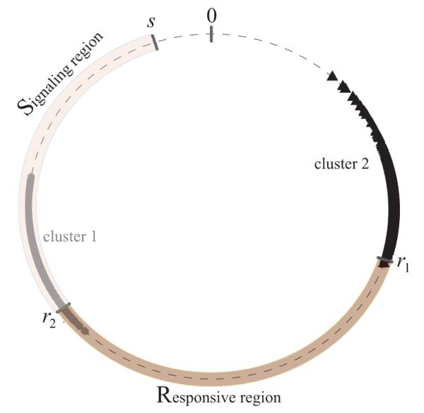
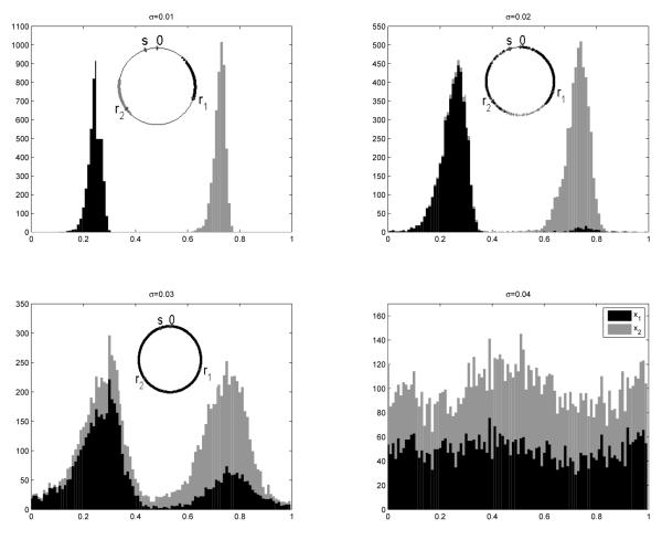
A snapshot of a two-cluster solution in the ensemble of n = 10⁴ cells represented on a unit circle. The coupling function is f(I) = −0.5I. The signaling region is S = [r₂, s] and the responsive region is R = [r₁, r₂] with r₁ = 0.3, r₂ = 0.65 and s = 0.95. Positions of the cells are indicated by grey circles and black triangles. Cells within clusters are spread because of Gaussian noise (the SDE model) added to the system.

Probing the biological details of the cell cycle is a topic of intense and fruitful study and many of the mechanisms involved in regulating the cell cycle within a cell are well-understood (see [15]). Our mathematical model obviously does not directly take into account any of this biology, but because of its universal nature, it can shed light on the biology when paired with experimental data.

We have considered the variation of the size and position of S and R in [5] and [26]. Let M = (|R + |S|)⁻¹ where |R| is the length of the responsive region and S is the length of the signaling region, we showed that this M is the maximum number of non-interacting clusters. For negative coupling, the clusters form only in numbers of at least M + 1. For any values of |R| and |S| with |R| + |S| < 1, we can find M + 1 periodic solutions which are stable under any negative coupling. In this manuscript, we consider only two-cluster periodic stable solutions and so we have chosen parameter values where 0.5 < |R| + |S| ≤ 1 and negative coupling.

Note that the form of coupling used in the model is instantaneous, i.e. there is no time delay between production and effect of the signal. Estimates show that chemical diffusion between cells in a stirred bioreactor is much faster than the progress of cells in the cell cycle [9]. Elsewhere, we have considered a model with an explicit term to represent the signaling agent [6] and a model with a gap between R and S [9]. For both models we showed that a time delay does not affect the qualitative global dynamics, but rather enhances the stability of stable clustered periodic solutions.

Budding yeast divides asymmetrically resulting in distinguishable mother and daughter cells. Because daughter cells are smaller than their mothers at division, they have a longer time to maturity and thus a longer cell cycle. These differences disperse the cell cycle synchrony of an initially synchronous population [21, 25] and complete population synchrony is generally impossible to maintain in the laboratory [4, 13, 24]. We refer to this mechanism of population dispersion as asymmetric division. Versions of this mechanism were studied in [8, 10] where, in the absence of coupling, it was shown to lead to a globally attracting steady state (with cells progressing around the cycle, but the distribution is time-independent).

In addition to asymmetric division, physical variation and epigenetic differences among the isogenic cells may produce small variations in growth rate. In [1], several scenarios of this are discussed. One may model this by adding Gaussian white noise, which is described by a system of coupled stochastic differential equations (SDEs). In the following we call this the SDE model. The SDE model lacks strict biological basis and suffers from the non-biological consequence that cells may, for short periods, grow at unrealistic rates or even “grow” backwards. However, stochastic perturbations are convenient because of the well developed methods for studying such models.

In a third model we will consider a more biologically reasonable model representing the unavoidable small inhomogeneity among cells. When each cell begins its cycle (at division) it will be randomly and independently assigned a rate of progression that is a small and bounded perturbation from the mean rate of the ensemble. We call this the variable rate model.

Note that asymmetric division and variable rate models are both examples of perturbations by bounded noise (see [11, 12, 27]). It is known that random differential equations with bounded noise may undergo discontinuous bifurcations of their minimal forward invariant (MFI) sets. MFI sets are the bounded noise analogue of attractors [12]. Namely, if there is a topological change in the collection of MFI sets, this change must be discontinuous (with respect to the Hausdorff metric on sets) [14]. One motivation for our study is to determine how such bifurcations may influence observed dynamics in biologically derived forms of bounded noise.

2 Perturbed models and numerical integration

2.2 Variable rate model

Considering the epigenetic differences and physiological variations among the isogenic cells which may produce small variations that favors population diffusion [1], we propose the following perturbed coupling model:

$$\frac{{\mathit{dx}}_k}{\mathit{dt}}=\{\begin{array}{cc}1+U_k\left(t\right),\hfill & \mathrm{if}{x}_k\notin R\hfill \\ 1+U_k\left(t\right)+f\left(I\right),\hfill & \mathrm{if}{x}_k\in R,\hfill \end{array}\phantom{\}}$$

(2.2.2)

where U_k(t) is a uniformly distributed random variable, $U_k\left(t\right)\in [-\sqrt{3}\sigma ,\sqrt{3}\sigma ]$, with the standard deviation (SD) σ. The variables {U_k(t), k = 1, , n} are taken to be independent and identically distributed and satisfy U_kU_k’ = δ_k,k’σ². For the k-th cell, variable U_k(t) remains constant within each cycle and is updated when the k-th cell passes through its division at 1 ~ 0.

We integrate (2.2.2) numerically by the Euler method,

$$x_k^{j+1}=x_k^j+h\left[a(x_k^j,I_j)+U_k^j\right],$$

where $U_k^j$ is updated when x_k crosses 1. Figure 2 shows the distributions of the cells in the variable rate model for several values of the noise SD, σ.

Open in a separate window

Figure 2

Steady-state distributions of two clusters in the variable rate model of noise for the indicated values of σ. Insets show positions of cells on the circle with indicated signalling (S) and responsive (R) regions.

3 Simulations and statistical measures

Throughout the simulations we set the coupling term to be linear and negative, f(I) = −αI, where the parameter α determines the coupling strength. In the following we fixed α = 0.5 and simulated an ensemble of n = 10⁴ cells which were initially distributed in two clusters at $x_k={\stackrel{‒}{x}}_1=\frac{1}{4}$ for $k=1,..,\frac{n}{2}$ and $x_k={\stackrel{‒}{x}}_2=\frac{51}{70}$ for $k=\frac{n}{2}+1,\dots ,n$, i.e. at the values of the two-cluster periodic solution of the deterministic system (see Appendix A).

The collective dynamics of the cell ensemble are conveniently described on a unit circle, so that the probability density function of the ensemble p(t, x) are periodic, i.e. p(t, x) = p(t, x + 1). The second Fourier harmonic of such a distribution is,

where V₂(t) is also known as the resultant vector in context of circular statistics. In Eq.(3.3.1) the averaging, ·, is taken over the entire ensemble, $\langle \cdot \rangle \equiv (1∕n){\sum }_{k=1}^n[\cdot ]$. The magnitude of the second harmonic, L₂(t) = |V₂(t)|, which we call the order parameter,

serves as a measure of phase coherence of the two-cluster solution. For the deterministic case the probability density is the sum of two delta functions, $p\left(x\right)=0.5\left[\delta \right(x-{\stackrel{‒}{x}}_1)+\delta (x-{\stackrel{‒}{x}}_2\left)\right]$, L₂ attains its maximal value near 1 (it is not exactly 1 since in the periodic solution the phase difference of the clusters is not exactly π). In the opposite limit of a disordered state with a uniform distribution, the order parameter is 0, i.e. L₂ = 0.

Noise-induced spread of a single cluster can be analyzed, with angular deviation defined as follows. We introduce the resultant vector for the first cluster,

where the averaging, ·₁, is taken only over the cells which were initially in that cluster, i.e. ${\langle \cdot \rangle }_1\equiv (2∕n){\sum }_{k=1}^{n∕2}[\cdot ]$. Then, the angular deviation is

attaining values from 0 (delta-peaked cluster) to $\sqrt{2}$ (uniform distribution).

In addition to circular statistics measures above, we have characterized the shape of the steady state probability distribution p(x) using a normalized entropy, E. Numerically, we used M = 100 partitions to estimate p(x) and its Shannon entropy, $H=-{\sum }_{m=1}^M{p}_m\log p_m$. In the absence of noise, the two-cluster solution is characterized by a double delta-peaked distribution and the entropy takes its minimal value, H_min = log 2 for symmetrical clusters with n/2 cells in each. In the completely disordered state the distribution p(x) is uniform with the maximal possible entropy H_max = log M. The normalized entropy defined as,

varies between 0 (noiseless two symmetrical clusters) and 1 (disordered state, cells are distributed uniformly).

For a given value of noise strength, σ, the ensemble “thermalizes” – evolving towards a steady state, which we characterized by two methods. The first method was based on comparison of the ensemble distributions at consecutive times when the ensemble was at a given position on the cycle. In particular, snapshots of the ensemble were taken at moment of times when the imaginary part of the ensemble’s second harmonic, sin[4πix_k(t)], was crossing zero with a negative slope. A two-sample Kolmogorov-Smirnov (K-S) test was used to probe whether the ensemble distribution settled down to its steady state. In the second method we used convergence to a steady state values of the circular measures, L₂(t) and D_c(t), introduced above. As we show further on, for all the three models, the relaxation time for the ensemble to reach its steady state is less than 100 cycles, except for a critical noise strength at which clusters are destroyed completely. Because of periodicity of the two-cluster solution and finite size fluctuations, the ensemble-averaged measures L₂, D_c and E are time-dependent even in the steady state. We thus performed additional time averaging of L₂, D_c and E over T = 100 after the ensemble reached its steady state, resulting in time-averaged quantities, ${\overline{L}}_2$ and ${\overline{D}}_c$ and $\overline{E}$.

Representative examples of steady-state distributions for individual clusters are shown in Figure 2. For weak noise (σ [0.01, 0.02]) the ensemble converges to the steady state in less than 20 cycles, according to the K-S test. For larger noise, σ > 0.025, convergence is slower, in about 80 cycles.

4 Results

4.1 Transient dynamics

Figure 3 shows that the ensemble distributions taken at a fixed position on the cycle (see previous section) evolves towards steady states for the SDE model. Weak noise (σ = 0.01) results in spread of cells within each cluster with extremely rare transitions of cells between clusters. Clusters still exist for an intermediate noise (σ = 0.02), although cells migrate between clusters, which is indicated by appearance of non-zero probability between peaks in the time-dependent probability map (middle panel of Figure 3). For σ > 0.04 the clusters are destroyed by the noise, so that the ensemble quickly approaches a steady state with a uniform distribution.

Open in a separate window

Figure 3

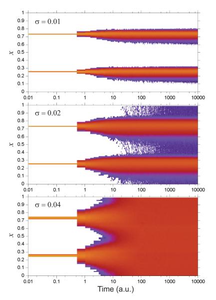
Time-dependent probability distributions p(t, x) of the ensemble with Gaussian white noise (SDE model) for the indicated values of noise strength σ. Logarithm of the probability distribution, log[p(t, x)], is shown as filled contours.

The transient dynamics are characterized further in Figure 4. Both the order parameter, L₂(t), and angular displacement of individual clusters, D_c(t), show characteristics approaching the steady state which are similar for all three models of noise. For small (σ < 0.03) and large (σ > 0.04) noise the order parameter and angular displacement settle to steady states within 100 cycles. However, for a critical noise strength (σ ≈ 0.035 for the SDE, σ ≈ 0.034 for uniform and σ ≈ 0.04 for the Bernoulli noise model) the relaxation process slows down dramatically and shows larger fluctuations in the steady state, indicating occurrence of a phase transition (bifurcation) from the ordered state with two clusters to the completely incoherent disordered state of the ensemble.

Open in a separate window

Figure 4

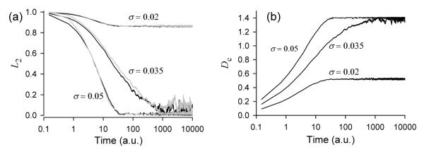
Time-dependence of (a) the order parameter, L₂(t), and of (b) the angular deviation, D_c(t), for the indicated values of noise strength σ in the SDE model. For a comparison, the corresponding dependencies L₂(t) for the variable rate model are shown by grey lines on panel (a). The values of noise standard deviations are the same as for the SDE model, except for the middle grey curve, where the noise standard deviation is 0.034.

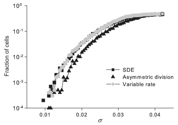
For the SDE model, the cell migration between clusters is expected for any non-zero noise intensity with exponentially long waiting time. On the contrary, for bounded noise models (variable rate and asymmetric division) there is a critical noise intensity, σ_h at which a “hard” bifurcation occurs [11]. For σ < σ_h cells are stuck within clusters, while for σ > σ_h cells can migrate between the clusters. Figure 5 shows the fraction of migrated cells after the ensemble evolves over 80 cycles, versus noise strength. As expected, the fraction of migrated cells grows with σ for all three models, saturating to 1/2 at the disordered state of the ensemble. Analytical calculations presented in Appendix B show that for the parameter values used, the hard bifurcation occurs at σ_h ≤ 1.4 × 10⁻⁵, which is far below the noise level where cells migration can be possibly observed for a reasonable integration time. We thus conclude that the hard bifurcation plays no essential role in these examples of biologically motivated noise.

Open in a separate window

Figure 5

Fraction of cells that have escaped from their initial clusters after 80 cycles for the three models. For noise levels below σ ≈ 0.01 cells are effectively bound to their cluster by the asymptotic stability of the two-cluster solution.

4.2 Sensitivity to noise and order-disorder phase transition

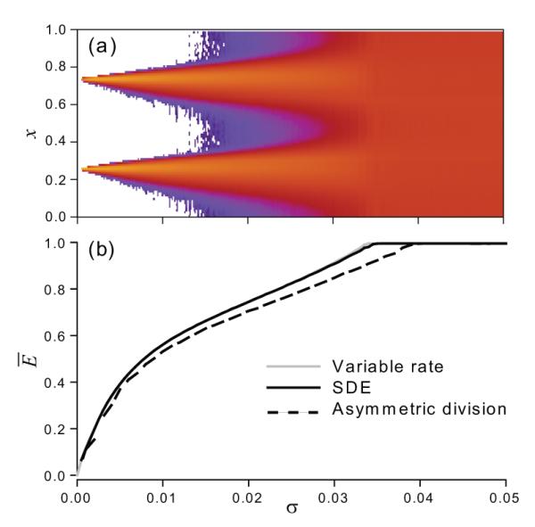
With the increase of noise strength the clusters exist until σ reaches its critical value above which the ensemble assumes a disordered state where no clustering can be distinguishable, as shown in Figure 4.2(a). This change of shape of the steady state distribution is well reflected by the normalized entropy, E, which increases from 0 (no noise) and reaches its maximal value when the ensemble distribution becomes uniform, Fig. 4.2(b). We can also see from this figure that the three models show qualitatively identical behaviour vs noise strength as to the distribution of the ensemble. The width of the clusters increases with the increase of noise SD, which is characterized by the order parameter and angular deviation shown in Figure 7(a,b). The order parameter decreases with the increase of noise until σ reaches a critical value, σ_c, at which ${\overline{L}}_2$ vanishes.

Open in a separate window

Figure 7

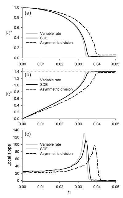
Stationary statistical measures of the cell ensemble versus noise strength σ for the three noise models. (a) Time averaged order parameter, ${\overline{L}}_2$, vs noise standard deviation, σ, of the three models. (b) Time averaged angular deviation of the first cluster vs σ. Dotted line shows the maximum possible value of $\sqrt{2}$. (c) Local slopes of angular deviations estimated from the curves in panel (b).

The spread of cells in clusters is best described by the angular deviation ${\overline{D}}_c$, which increases with the increase of noise and reaches its maximum value $\sqrt{2}$ at the transition point. The dependencies ${\overline{D}}_c\left(\sigma \right)$ in Figure 7(b) show three distinct regions of noise SD. For weak noise, σ < 0.015, the angular deviation increases linearly with σ, indicating a linear response of the ensemble to noise perturbations. Linear response is broken for intermediate noise whereby ${\overline{D}}_c$ non-linearly increases with progressively larger slopes. For strong noise, σ > σ_c, ${\overline{D}}_c$ saturates to its maximum value. This is further illustrated in Figure 7(c) by local slopes of ${\overline{D}}_c$ vs σ dependencies, which clearly shows the regions of linear and non-linear responses. We note that the local slope is a measure of sensitivity of the ensemble to noise perturbations and it shows that this sensitivity is maximal near the transition to the disordered state.

For σ > σ_c, i.e. in the disordered state, the ensemble is insensitive to noise perturbations, as indicated by the zero slope of ${\overline{D}}_c\left(\sigma \right)$.

Figure 7 further indicates that the three noise models show qualitatively identical dependencies versus noise SD, σ. Quantitatively, however, the asymmetric division model shows consistently lower sensitivity to noise perturbations. We note that while in the SDE and variable rate models noise is applied throughout the whole cycle, the asymmetric division model is perturbed by Bernoulli noise once per cycle only. Hence an effective noise strength of the SDE and variable rate model is larger than that of the asymmetric division model. Furthermore, because the distribution of cells in asymmetric division model always has a higher density in the interval [1 – 2σ, 1] in phase space the order parameter saturates to a non-zero value for large σ in Fig.7(a).

At the critical value of noise SD, σ = σ_c, the ensemble demonstrates features of an order-disorder phase transition, such as slowdown of transient relaxation to the steady state and large fluctuations (see Figure 4). The transition of the distribution of the solution has the characteristics of an Andronov-Hopf bifurcation, as indicated by Figure 8. For σ < σ_c the model possesses a stable limit cycle that bifurcates to a stable focus for σ > σ_c. Here the large noise effectively stabilizes the uniform solution, which otherwise is unstable. Further, in Figure 7(a) we observe that the amplitude of the periodic orbit has a square root type dependency on σ, as in a Hopf bifurcation. We note here that this transition is consistent with order-disorder transitions in theKuramoto model of globally coupled stochastic phase oscillators [18]. There the rotation of the original variables has been discarded by the transformation to phase differences, so the linearization there has zero imaginary part at the bifurcation.

Open in a separate window

Figure 8

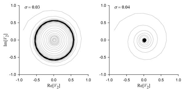
Phase portraits of the SDE model projected onto the complex plane of the second Fourier harmonic. Black lines show steady state trajectories; grey lines show transients on both panels. Left: two-cluster ordered state, with a stable periodic orbit, σ = 0.03. Right: stable equilibrium distribution at the disordered state, σ = 0.04. The order-disorder transition occurs at σ_c ≈ 0.035.

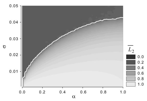
The critical noise strength, σ_c, is indeed a function of the coupling strength, α. Figure 9 shows that a stronger coupling requires stronger noise to destroy the two-cluster ordered state. The white curve in this graph corresponds to a bifurcation line separating ordered and disordered states in the (α, σ) parameter plane. The region below the white curve represents cells in the two-cluster ordered state, possessing a limit cycle. While the region above the white curve represents cells in disordered states, which is a stable uniform solution. This curve is also consistent with phase transitions observed in globally coupled stochastic phase oscillator systems [18].

Open in a separate window

Figure 9

Time averaged order parameter, ${\overline{L}}_2$, as a function of the coupling strength, α, and noise SD, σ.

5 Yeast cultures have large coupling mechanisms

In budding yeast, a mother cell carries a scar from the bud and the daughter does not. Replicative age can be determined from the number of scars [19]. A natural phase space for a model stratified by replicative age is to represent the cell cycle of the daughters by I₀ = [0, 1] and successive generations by I_m = [a_m, 1]. In other words, the phase space is: I₀ I₁ I_n where n is the highest generation considered. In a steady state bioreactor, the fraction of cells in each generation decreases roughly geometrically with age, so n does not need to be large for accurate modeling.

Denote τ_m = |I_m| = 1 – a_m. The age distribution can be measured and is directly related to the relative lengths of the cell cycles τ_m [2]. For one autonomous oscillation experiment in which clustering was detected we determined the following population fractions as a function of generation for the first four generations: 0.55, 0.24, 0.11, 0.05 [2]. The corresponding τ_m’s are calculated to be: 1.0, 0.93, 0.86, 0.82, so we find:

In [2, 22] we showed that simulations using these proportions can accurately reproduce the behavior seen in the YAO experiment [3, 22]. A standard calculation shows that the standard deviation of the generational noise, σ_g, in the experiment is:

This quantity is normalized to a time unit of one cell cycle in the experiment.

In Figure 9, we see that for σ ≈ 0.036 a coupling coefficient of α > 0.6 is needed for the coupling strength to overcome the dispersive action of the asymmetric division and produce detectable clustering. Consider that the units here are all normalized in terms of one unperturbed cell cycle. We can conclude that for clustering to exist in the autonomous oscillation experiment, as observed, the strength of coupling must be a rather large effect. In a two-cluster state, the clusters as they enter the region where they experience coupling, need to have their rate of progression decreased by a normalized factor of at least 0.3, or, 30%. Such a decrease cannot be considered to be a small perturbation.

6 Conclusions

We have studied the effects of two biologically motivated dispersive mechanisms, as well as standard Gaussian white noise, in an ensemble cell cycle coupling model that successfully predicts clustering behavior observed experimentally.

One conclusion for this simple generic model is that the difference between biologically plausible bounded noise and Gaussian noise mechanisms is insignificant after proper scaling of the noise strength. This is observed in both the ensemble statistics of the clusters and in terms of the expected phenomena of bounded noise dynamics. As seen in Figure 7, asymmetric division and variable rate perturbations lead to circular statistics measurements that are indistinguishable from the results using Gaussian white noise perturbations. Further, the theory of bounded noise dynamical systems predicts that cells will be unable to escape a stable cluster for noise levels below some threshold. However, we observe in this application that the threshold is far too small to play a role in observed behavior. For such small values of noise, the expected time to escape would be extremely long for the Gaussian noise model and so there is no observable difference.

For all three forms of applied noise perturbations the dispersion of clusters occurs in three distinct phases. First, for small noise there is a linear relationship between the noise level and the dispersion of the clusters measured by the circular angular deviation. In this phase cells do not migrate from their initial clusters on the time scales considered. In the second phase cells begin to migrate more frequently between clusters and the slope of the dispersion versus noise increases. Finally, for noise level above a certain threshold the clustering structure is destroyed and the cells assume a nearly uniform distribution. This phase transition between disorder and order exhibits many characteristics of a Hopf bifurcation, e.g. the birth of a stable limit cycle out of a stable equilibrium and a square-root dependence of the amplitude of the periodic orbit on the bifurcation parameter (noise strength).

Finally, we conclude that the clustering observed in autonomous oscillation experiments cannot be due to small coupling effects. When we compare experimental data with the transition from clustered to uniform distribution in Figure 4.2, we can see that the experimentally established level of dispersion due to asymmetric division alone is enough to require a coupling strength at least strong enough to produce a 30% relative decrease in rate of progression when a cell enters the responsive region. Although the model is minimal, it is both universal and normalized to the length of the unperturbed cell cycle, so this estimate of relative effects of noise and coupling is reliable. One possible explanation for a coupling strength of this magnitude is that the mechanism actually involves one or more check points in the cycle.

Acknowledgements

Appendix A. Calculation of the two-cluster periodic solution

In this appendix we derive the exact initial conditions for the periodic two-cluster solution of the unperturbed (no noise) model.

Recall that the responsive region has coordinates R = [0.3, 0.65] and the signaling region is S = [0.65, 0.95]. The coupling function is f(I) = −αI, with α = 0.5 in our computations. We know from [26] that a periodic two-cluster solution exists and that for these parameter values it must be stable.

Let the initial condition of the first cluster be $x_1\left(0\right)=\frac{1}{4}$ and the initial condition of second cluster be denoted as x₂(0) which is near (but not exactly) 0.75 and inside S. The calculation of the solution depends on the “order of events.” Namely, from [5] we know that x₁(t) must enter R while x₂(t) is still in S and then x₂(t) must leave S while x₁(t) is still in R. With these facts in mind we may calculate exactly the trajectory of the clusters starting from our initial condition (1/4, x₂(0)) as follows.

• x₁ enters the responsive region, i.e. x₁ = 0.3. When x₁ reaches 0.3, we have x₁(t₁) = 0.3. It is then easy to solve for

  $$t_1=x_1\left(t_1\right)-x_1\left(0\right)=\frac{1}{20}.$$

  Since x₂ is progressing with rate 1 during this phase, $x_2\left(t_1\right)=x_2\left(0\right)+t_1=x_2\left(0\right)+\frac{1}{20}$.

• x₁ experiences coupling before x₂ leaves the signaling region, i.e. until x₂ = 0.95.

  Assume t₂ is the time when x₂ leaves the signaling region, then x₂(t₂) = 0.95. Since x₂ travels at a constant rate 1, we have

  $$t_2=x_2\left(t_2\right)-x_2\left(0\right)=\frac{19}{20}-x_2\left(0\right).$$

  However, x₁ is slowed by the coupling function $f\left(\frac{1}{2}\right)=-\frac{1}{4}$, so

  $$x_1\left(t_2\right)=x_1\left(t_1\right)+\left(1+f\left(\frac{1}{2}\right)\right)(t_2-t_1)=\frac{3}{10}+\frac{3}{4}(\frac{9}{10}-x_2(0\left)\right)=\frac{39}{40}-\frac{3}{4}{x}_2\left(0\right).$$

• x₂ arrives at $x_1\left(0\right)=\frac{1}{4}$ and because this is the periodic solution, x₁ reaches x₂(0).

  During this phase, there is no coupling exerted. Thus the time t₃ for $x_3\left(t_3\right)=\frac{1}{4}$ can be found by:

  $$t_3=t_2+\left(x_2\right(t_3)+1-x_2(t_2\left)\right)=\frac{19}{20}-x_2\left(0\right)+\frac{1}{4}+1-0.95=\frac{5}{4}-x_2\left(0\right).$$

  At this time,

  $$x_1\left(t_3\right)=x_1\left(t_2\right)+(t_3-t_2)=\frac{39}{40}-\frac{3}{4}{x}_2\left(0\right)+\frac{3}{10}=x_2\left(0\right).$$

  We may solve the above equation to find that $x_2\left(0\right)=\frac{51}{70}$.

We can also obtain from the above calculations that $t_3=\frac{5}{4}-x_2\left(0\right)=\frac{73}{140}$.

Thus the period for this two-cluster periodic solution is $T_2=2t_3=\frac{73}{70}>1$. This is slightly larger than 1 as should be expected for negativecoupling.

Appendix B. Hard bifurcation for the bounded noise system

We will derive an upper bound on the noise level σ at which a hard bifurcation must occur. We first observe that in our negative coupling model “back stability” is much weaker than front stability. The reason for this is that when a nearly synchronized group of cells crosses the boundary from R to S the cells in the front of the group begin to add to the negative coupling in R before the trailing cells leave R.

Consider the variable rate model and first set the noise equal to 0. Now consider the two-cluster periodic solution (i.e. with x₁(0) = 1/4 and x₂(0) = 51/70), but perturb the solution by removing one cell from the cluster at 1/4, and placing it at 1/4 – . Denote the state of this cell by x₁. We may calculate the trajectory starting at this initial condition exactly, using the same procedure as in the previous section.

1. x₁ reaches R before x₂ gets out of S, i.e. x₁ = 0.3.

   At this time, x₂ = 109/140 and x₁ = 0.3 – .

2. x₁ reaches at R before x₂ gets out of S, i.e. x₁ = 0.3. During this period, only x₁ is experiencing coupling f(I) = −0.5I = −1/4 because x₂ is in the signaling region. So x₁ = 0.3 + 0.75 and x₂ = 109/140 + .

3. x₂ gets out of S while x₁ and x₁ are still in R, i.e. s₂ = 0.95. During this phase, both x₁ and x₁ are affected by the couping. The time for x₂ to reach at 0.95 is 6/35 – . Thus at this time, x₁ = 0.3 + 0.75+(6/35–)0.75 = 3/7 and x₁ = 0.3+(6/35–)0.75 = 3/7–0.75.

4. x₁ gets out of R and arrives at S while x₁ is still in R, i.e. x₁ = 0.65. No coupling is exerted. So we have when x₁ reaches 0.65, x₂ = 0.95 + 31/140 mod 1 = 6/35 and x₁ = 0.65 – 0.75.

5. x₁ reaches at S as well, i.e. x₁ = 0.65.

In this case, x₁ is in S and x₁ is in R. Thus the coupling function is $f\left(I\right)=-0.5\frac{4990}{10000}=-0.24995$. The time for x₁ to arrive at 0.65 is $0.75∊∕(1-0.24995)=\frac{15000}{15001}∊$. So we have $x_1=0.65+\frac{15000}{15001}∊$.

After the first cluster and the cell both get out of R, we find the distance between them is $\frac{15000}{15001}∊$, which was initially . This spacing will persist as the cluster x₁ returns to 1/4, so the distance is decreased by a factor of 15000/15001. Thus we see that the stability of the solution is very weak with respect to this particular perturbation.

To consider how noise breaks this stability, perform the following perturbations which are a possible realization of the variable rate model. Let x₁ progress at a constant rate of 1 + σ, the single cell at a rate of 1 – σ, and x₂ progress at rate 1. Denote $\beta =f\left(\frac{1}{2}\right)$ and $\widehat{\beta }=f\left(\frac{4,999}{10,000}\right)$ where f(I) = −0.5I. The cell at x₁ and the cluster x₁ are progressing at different rates and therefore constantly drifting apart, except while the coupling strength is pulling them together. We will make a simplifying assumption here that we consider the drift only during the periods when x₁ and x₁ are experiencing different strength of coupling. This is fine since we are only looking for an upper bound on the bifurcation value.

Considering a complete cell cycle of the cluster and the cell, there are three stages when they experience different coupling:

1. When the 4,999-cell cluster x₁(t) enters R, but x₁ has not yet entered R, the second cluster x₂(t) is still in S, so the coupling β only affects x₁. It takes the cell x₁ time $\frac{∊}{1-\sigma }$ to enter R. At this time, the distance between x₁ and x₁(t) is $\frac{1+\sigma -\beta }{1-\sigma }∊$.

2. When the x₁(t) and the cell x₁ both lie in R and the second cluster is still in S, both of the broken cluster and the cell experience the coupling β. We neglect the changing of the distance between the cell and the cluster during this time by our simplifying assumption.

3. When the cell x₁ lies in R and x₁ enters S, we know the second cluster is not in S. Hence the coupling strength the cell experiences is $\widehat{\beta }$. The time from the cluster enters S to the cell enters S is $\frac{1}{1-\sigma +\widehat{\beta }}\frac{1+\sigma -\beta }{1-\sigma }∊$, thus the distance between the cell and the cluster after the cell enters S is $\frac{1+\sigma }{1-\sigma +\widehat{\beta }}\frac{1+\sigma -\beta }{1-\sigma }∊$.

Setting the coefficient $\frac{1+\sigma }{1-\sigma +\widehat{\beta }}\frac{1+\sigma -\beta }{1-\sigma }$ equal to 1, we calculate σ = .000014. For this amount of noise, the original distance between cell and the broken cluster will stay the same. Any more noise will increase the initial distance.

The calculations above assume that we are near the cyclic solution. In our calculations during stage 1, we assumed that when the cluster entered R, the second (unbroken) cluster was in S, and remained there until after the isolated cell entered R. In the calculations in stage 3, we assumed that the single cell reached 1 before the broken cluster entered S again. When the cell is pulled sufficiently far from the broken cluster due to the noise, the assumption in stage 1 breaks down. We next calculate the distance if this happens.

Consider the unperturbed model again. The threshold occurs when the broken cluster lies at .65, the nonbroken cluster lies at .12858, and the cell lies at .47858. Move the cell back to .47858 – , and denote the distance between cluster and cell as $\widehat{∊}$. Then initially, $\widehat{∊}=.17142+∊$. Run time until C₁ = .3, C₂ = .77857, and c = .64 – ; now $\widehat{∊}=.12857+∊$. Advance time further so that C₂ = 1 and c = .87143 – ; at this time $\widehat{∊}=.12857+∊$. Running time until c = 1, we obtain $\widehat{∊}=.17142+1.3332∊$.

So even in the non-perturbed model, once the cell has achieved a sufficient separation from the cluster, the distance will widen; we do not need noise beyond σ = .000014 that we initially obtained. The hard bifurcation, below which cells have no possibility to escape their initial cluster, is below the value .000014. While this rigorous upper bound on the bifurcation is quite rough, we see in Figure 5 that it is already far lower than noise levels for which an escape can actually be observed.

Footnotes

References