Abstract
Free full text

Multi-trait analysis of genome-wide association summary statistics using MTAG
Abstract
We introduce Multi-Trait Analysis of GWAS (MTAG), a method for joint analysis of summary statistics from GWASs of different traits, possibly from overlapping samples. We apply MTAG to summary statistics for depressive symptoms (Neff = 354,862), neuroticism (N = 168,105), and subjective well-being (N = 388,538). Compared to 32, 9, and 13 genome-wide significant loci in the single-trait GWASs (most of which are themselves novel), MTAG increases the number of loci to 64, 37, and 49, respectively. Moreover, association statistics from MTAG yield more informative bioinformatics analyses and increase variance explained by polygenic scores by approximately 25%, matching theoretical expectations.
INTRODUCTION
The standard approach in genetic-association studies is to analyze a single trait. Such studies do not exploit information contained in summary statistics from genome-wide association studies (GWASs) of related traits. In this paper, we develop a method, Multi-Trait Analysis of GWAS (MTAG), which enables joint analysis of multiple traits, thus boosting statistical power to detect genetic associations for each trait.
Compared to the many existing multi-trait methods,1–5 MTAG has a unique combination of four features that make it potentially useful in many settings. First, it can be applied to GWAS summary statistics (without access to individual-level data) from an arbitrary number of traits. Second, the summary statistics need not come from independent discovery samples: MTAG uses bivariate linkage disequilibrium (LD) score regression6 to account for (possibly unknown) sample overlap between the GWAS results for different traits. Third, MTAG generates trait-specific effect estimates for each single-nucleotide polymorphism (SNP). Finally, even when applied to many traits, MTAG is computationally quick because every step has a closed-form solution.
The MTAG estimator is a generalization of inverse-variance-weighted meta-analysis that takes summary statistics from single-trait GWASs and outputs trait-specific association statistics. The resulting P values can be used like P values from a single-trait GWAS, e.g., to prioritize SNPs for subsequent analyses such as biological annotation or to construct polygenic scores.
The key assumption of MTAG is that all SNPs share the same variance-covariance matrix of effect sizes across traits. This assumption is strong and is violated in many circumstances, most intuitively in scenarios where some SNPs influence only a subset of the traits. Even if this assumption is not satisfied, however, we show analytically that MTAG is a consistent estimator and that its effect estimates always have a lower genome-wide mean squared error than the corresponding single-trait GWAS estimates. Hence, polygenic scores constructed from MTAG results are expected to outperform GWAS-based predictors very generally.
The main potential problem arises for SNPs that are truly null for one trait but non-null for another trait. For such SNPs, MTAG’s effect-size estimates for the first trait are biased away from zero, leading to an increased rate of false positives (and inflated type I error rate). We derive an analytic formula for the resulting false discovery rate (FDR), given any specified mixture-normal distribution of effect sizes (including multivariate spike-and-slab distributions), and we illustrate how the formula can be used to probe the credibility of MTAG-identified loci.
To demonstrate the utility of MTAG empirically, we analyze three traits: depressive symptoms (DEP, Neff = 354,862), neuroticism (NEUR, N = 168,105), and subjective well-being (SWB, N = 388,538). Prior GWASs of each of these traits have identified only a handful of loci.7–11 Because of the high genetic correlations between the three traits—in our data, roughly 0.7 in absolute value between each pair—some papers have conducted cross-trait analyses to replicate findings for one of the traits11 or joint meta-analysis to identify new loci.5 We apply MTAG to these traits because we expected the gains in power would be substantial, violations of MTAG’s assumptions would be limited, and the substantive results would be of interest.
Finally, we compare MTAG to the three existing multi-trait methods we are aware of that can be applied to GWAS summary statistics from an arbitrary number of traits with unknown sample overlap.12,13 We find that MTAG has greater power across a wide range of simulation scenarios and in two separate applications to real data.
RESULTS
Overview of MTAG
The key idea underlying MTAG is that when GWAS estimates from different traits are correlated, the effect estimates for each trait can be improved by appropriately incorporating information contained in the GWAS estimates for the other traits.
Correlation between GWAS estimates can arise for two reasons. First, the traits may be genetically correlated, in which case the true effects of the SNPs are correlated across traits. Second, the estimation error of the SNPs’ effects may be correlated across traits. Such correlation will occur if (a) the phenotypic correlations are non-zero and there is sample overlap across traits, or if (b) biases in the SNP-effect estimates (e.g., population stratification or cryptic relatedness) have correlated effects across traits. MTAG boosts statistical power by incorporating information about these two sources of correlation.
MTAG Framework
In the framework that follows, all traits and genotypes are standardized to have mean zero and variance one. For SNP j, we denote the vector of marginal (i.e., not controlling for other SNPs), true effects on each of the T traits by
We denote the vector of GWAS estimates of SNP j’s effects on the traits by
MTAG is the efficient generalized method of moments (GMM) estimator based on the moment condition
where
The MTAG estimator is a weighted sum of the GWAS estimates:
It is a consistent and asymptotically normal estimator for
There are several useful special cases of MTAG (Online Methods). When all estimates are for the same trait (implying
To make equation (1) operational, we use consistent estimates of
Estimation of
In standard meta-analysis, the diagonal elements of
Therefore, MTAG proceeds by running linkage disequilibrium (LD) score regressions14 on the GWAS results and using the estimated intercepts to construct the diagonal elements of
Estimation of
We estimate
with
Summary
The MTAG results for SNP j are obtained in three steps: (i) estimate the variance-covariance matrix of the GWAS estimation error,
Theoretical Analysis of MTAG’s Performance
This section briefly discusses three analytic formulas we have derived regarding the expected performance of MTAG for each trait: its mean squared error (MSE) across SNPs, its statistical power to detect a true single-SNP association, and its false discovery rate (FDR) (Online Methods). All the formulas hold for an arbitrary number of traits. Supplementary Note contains illustrative calculations.
The MSE formula is very general: it holds under any distribution of effect sizes, including distributions that violate the homogeneous-Ω assumption. The formula implies that for each trait, the MTAG estimates always have a lower genome-wide MSE than corresponding GWAS estimates. That in turn suggests that polygenic predictors constructed from MTAG results are likely to outperform GWAS-based predictors very generally.
The power and FDR formulas (in contrast to the fully general MSE formula) assume that the true effect sizes
Potential Biases in MTAG’s Test Statistics
The derivation of MTAG relies on three important assumptions: (1)
Homogeneous-
If the homogeneous-Ω assumption is violated, then there are different types of SNPs with different Ω’s. Because MTAG combines the GWAS estimates using the genome-wide (i.e., across-SNP) variance-covariance matrix, in general the MTAG estimates will be biased in finite samples. For a type of SNP that is null for one trait but non-null for other traits, the effect estimate on the first trait will be biased away from zero. For that reason, the FDR will be inflated.
Replication is the best way to assess the credibility of individual-SNP associations. In addition, their credibility can be probed using the FDR formula, computed under plausible assumptions about genetic architecture. In our application below, we calculate what we call maxFDR, which is an upper bound for the FDR under certain assumptions (Online Methods). In particular, we assume that the effect-size distribution is a multivariate spike-and-slab distribution in which at least 10% of SNPs are non-null for each trait. Illustrative calculations indicate that a trait’s maxFDR can become high when the GWAS for the trait is low powered while the GWAS for another trait is higher powered (Supplementary Note).
Sampling variation in
To assess the magnitude of the finite-sample bias in MTAG’s standard errors from ignoring sampling variation in
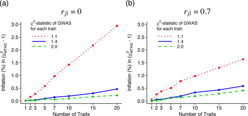
The y-axis is the percent increase in
(Figure 1a) or
These simulations suggest that in most realistic applications of MTAG, the bias from ignoring sampling variation in
MTAG relies on bivariate LD score regression (and by extension its assumptions) to estimate the correlation in GWAS estimation error due to sample overlap. To gauge MTAG’s performance, we simulate an extreme case of sample overlap using real data from the UK Biobank (UKB). We run three GWASs of height, each using two-thirds of the data, with 50% overlap between each pair of GWAS samples. Then we run MTAG on the three GWASs. Figure 2a is a scatterplot of the resulting MTAG z-statistics against the z-statistics from a single GWAS run on the entire UKB sample. Figure 2b is the scatterplot from an analogous analysis of DEP in UKB. The regression slope and R2 are both essentially one for both phenotypes, indicating that MTAG generates the correct z-statistics in these cases. The results are similar when we repeat this analysis using four other phenotypes (Online Methods).
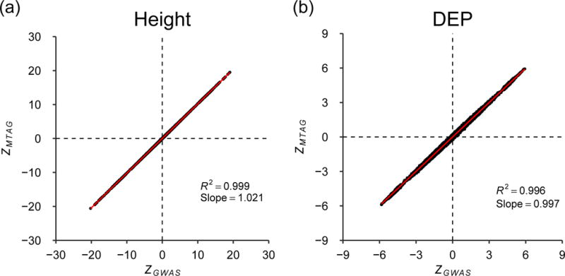
The x-axis is a SNP’s z-statistic from a baseline GWAS conducted in UK Biobank. The y-axis is a SNP’s z-statistic from applying MTAG to three GWASs of each trait conducted on equally sized subsamples of the baseline sample, in which every pair of samples has 50% overlap. (a) Height. (b) Depressive symptoms. The figure illustrates near-perfect alignment. See Supplementary Note for details and results from analogous analyses on additional phenotypes.
GWAS Summary Statistics for Depression, Neuroticism, and Subjective Well-Being
For our empirical application of MTAG, we build on a recent study by the Social Science Genetic Association Consortium (SSGAC) of three traits that have been found to be highly polygenic and strongly genetically related: depressive symptoms (DEP), neuroticism (NEUR), and subjective well-being (SWB). In these analyses, we combine data from the largest previously published studies7–9,11 with new genome-wide analyses from the genetic testing company 23andMe, Inc., and the first release of the UK Biobank (UKB) data. As depicted in Figure 3, there is substantial overlap between the estimation samples for the three traits. For additional details, see Online Methods and Supplementary Note.
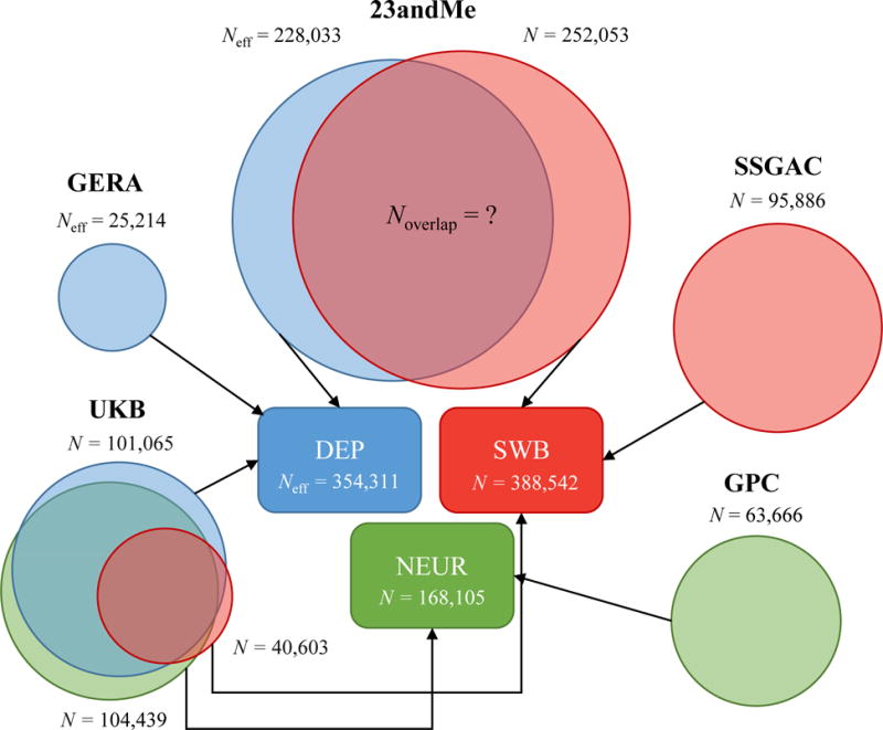
In UKB, the sample overlap in the summary statistics across the traits is known, whereas in 23andMe, the sample overlap in the summary statistics is unknown. MTAG accounts for both sources of overlap. SSGAC results,20 GPC results,19 GERA results,18 and 23andMe results for DEP21 all come from previously published work. The data from 23andMe for SWB are newly analyzed data for this paper. Data from the UKB for all three traits has been previously published,20 although we re-analyze it in this paper with slightly different protocols.
MTAG Results
We applied MTAG to the summary statistics from the three single-trait analyses described above. To enable a fair comparison between the MTAG and GWAS results, we restrict all analyses to a common set of SNPs (see Online Methods for details and recommended filters for MTAG).
Figure 4 shows side-by-side Manhattan plots from the GWAS and MTAG analyses for each trait. Approximately independent genome-wide significant SNPs, hereafter “lead SNPs,” were defined by clumping with an R2 threshold of 0.1 (Online Methods). From GWAS to MTAG, the number of lead SNPs increases from 32 to 64 for DEP, from 9 to 37 for NEUR, and from 13 to 49 for SWB.
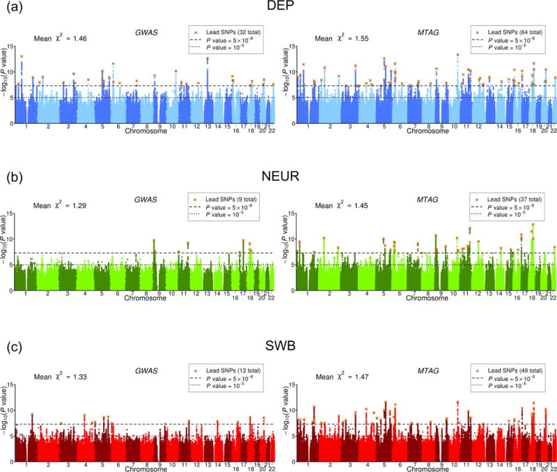
(a) DEP, (b) NEUR, (c) SWB. The left and right plots display the GWAS and MTAG results, respectively, for a fixed set of SNPs. The x-axis is chromosomal position, and the y-axis is the significance on a −
For the MTAG hits, we calculate the maxFDR assuming that at least 10% of SNPs are non-null for each trait (our estimates of the actual percentage non-null are 59-65% across the three traits; Online Methods). The maxFDR is 0.0014 for DEP, 0.0080 for NEUR, and 0.0044 for SWB. This calculation suggests that the hits are unlikely to be an artifact of the homogeneous-Ω assumption.
For each trait, we assess the gain in average power from MTAG relative to the GWAS results by the increase in the mean
Replication of MTAG-identified Loci
To test the lead SNPs for replication, we use the Health and Retirement Study (HRS) and the National Longitudinal Study of Adolescent to Adult Health (Add Health), which both contain high-quality measures of DEP, NEUR, and SWB. Because HRS was included in the SSGAC discovery sample for SWB, we re-ran the GWAS and MTAG analyses for SWB after omitting it. Although our replication samples are too small for well-powered replication analyses of single-SNP associations, we are well powered to test the SNPs jointly. For the set of MTAG-identified lead SNPs for each trait, we regressed the effect sizes in HRS and in Add Health on the MTAG effect sizes, after correcting the MTAG effect-size estimates for the winner’s curse (Supplementary Note). The regression slope for each replication cohort was then meta-analyzed. If the SNP effect sizes taken altogether replicate, then we expect a slope of one. The regression slopes are 0.88 (s.e. = 0.22) for DEP, 0.76 (s.e. = 0.21) for NEUR, and 0.99 (s.e. = 0.33) for SWB (Figure 5). In all cases, the slope is statistically significantly greater than zero (one-sided
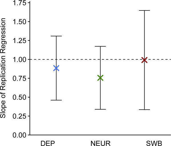
For each trait and in each of two independent replication cohorts (HRS and Add Health, combined N = 12,641), we regressed the estimated effect sizes of the MTAG-identified loci on their winner’s-curse-adjusted MTAG effect sizes. The intercept is constrained to zero in these regressions. The plotted regression coefficients are the sample-size-weighted means across the replication cohorts, with 95% intervals. See Supplementary Note for details and cohort-level results.
Polygenic Prediction
We next compare the predictive power of polygenic scores constructed from GWAS versus MTAG association statistics. We again use the HRS and Add Health as our prediction samples (and we obtain the SNP effect estimates for SWB from the analyses that omit HRS from the discovery sample).
We measure the predictive power of each polygenic score by its incremental
Figure 6 and Table 1 summarize the results from our pooled analysis of Add Health and HRS. The GWAS-based polygenic scores have incremental
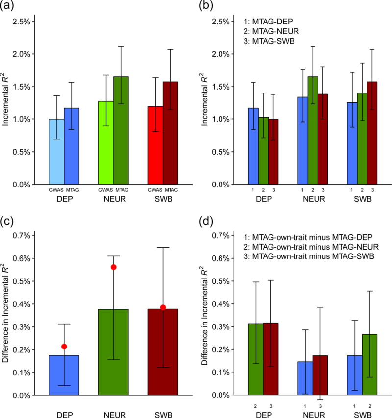
Incremental
Table 1
Summary of comparative analyses of GWAS and MTAG results
| DEP
| NEUR
| SWB
| ||||
|---|---|---|---|---|---|---|
| GWAS | MTAG | GWAS | MTAG | GWAS | MTAG | |
| SNP-based comparisons | ||||||
| Lead SNPs (P < 5×10⁻⁸) | 32 | 64 | 9 | 37 | 13 | 49 |
| Mean χ2 | 1.43 | 1.55 | 1.29 | 1.45 | 1.30 | 1.47 |
| Neff | 354,861 | 449,649 | 168,105 | 260,897 | 388,538 | 600,834 |
| Polygenic score incremental R2 | 1.00% | 1.17% | 1.27% | 1.65% | 1.20% | 1.57% |
| Biological Annotation (DEPICT FDR < 0.05) | ||||||
| # Prioritized Genes | 3 | 72 | 0 | 51 | 0 | 0 |
| # Gene Sets | 0 | 347 | 0 | 1 | 0 | 7 |
| # Tissues and cell types | 10 | 22 | 0 | 21 | 0 | 12 |
Biological Annotation
For a final comparison, we analyze both the GWAS and MTAG results using the bioinformatics tool DEPICT15. We present the prioritized genes, enriched gene sets, and enriched tissues identified by DEPICT at the standard FDR threshold of 5%.
Table 1 summarizes the results. In the GWAS-based analysis, very little enrichment is apparent. For DEP, 3 genes are identified, but no gene sets and only 10 tissues. For NEUR and SWB, no genes, gene sets, or tissues are identified. In contrast, the MTAG-based analysis is more informative. The strongest results are again for DEP, now with 72 genes, 347 gene sets, and 22 tissues. For NEUR, there are 51 genes, 1 gene set, and 21 tissues, and for SWB, zero genes, 7 gene sets, and 12 tissues.
For brevity, we discuss the specific results only for DEP; the results for NEUR and SWB are similar but more limited. For the tissues tested by DEPICT, Figure 7a plots the P values based on both the GWAS and MTAG results. As expected, nearly all of the enrichment of signal is found in the nervous system. To facilitate interpretation of the enriched gene sets, we used a standard procedure16 to group the 347 gene sets into ‘clusters’ defined by degree of gene overlap. Many of the resulting 46 clusters, shown in Figure 7b, implicate communication between neurons (‘synapse,’ ‘synapse assembly,’ ‘regulation of synaptic transmission,’ ‘regulation of postsynaptic membrane potential’). This evidence is consistent with that from the DEPICT-prioritized genes, many of which encode proteins that are involved in synaptic communication. For example, PCLO, BSN, SNAP25, and CACNA1E all encode important parts of the machinery that releases neurotransmitter from the signaling neuron.17
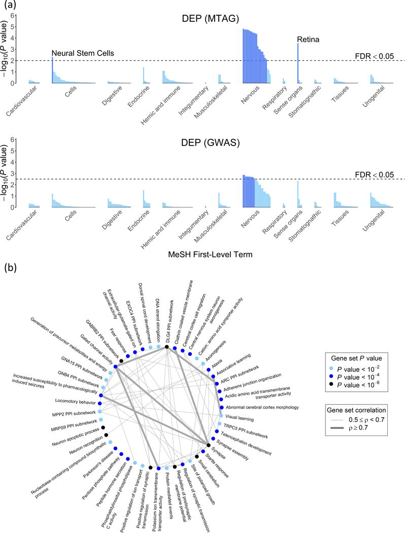
(a) Results of the tissue-enrichment analysis based on the GWAS and MTAG results. The x-axis lists the tissues tested for enrichment, grouped by the location of the tissue. The y-axis is statistical significance on a −
The results contain some intriguing findings. For example, while hypotheses regarding major depression and related traits have tended to focus on monoamine neurotransmitters, our results as a whole point much more strongly to glutamatergic neurotransmission. Moreover, the particular glutamate-receptor genes prioritized by DEPICT (GRIK3, GRM1, GRM5, and GRM8) suggest the importance of processes involving communication between neurons on an intermediate timescale,18,19 such as learning and memory. Such processes are also implicated by many of the enriched gene sets, which relate to altered reactions to stress and novelty in mice (e.g., ‘decreased exploration in a new environment,’ ‘increased anxiety-related response,’ ‘behavioral fear response’).
Comparison to Other Multi-Trait Methods
We compared MTAG to three multi-trait methods that can be applied to an arbitrary number of GWAS summary with unknown overlap12,13 (Supplementary Note). Unlike MTAG, these methods do not provide trait-specific SNP effect estimates but instead test whether the SNP is associated with none of the traits. We generate a (conservative) MTAG-based test of the same null hypothesis by using the minimum of the trait-specific MTAG P values, Bonferroni-adjusted for the number of traits. In two-trait simulations, we find that MTAG has greater power when the correlation in true effect sizes or GWAS estimation error is non-zero, especially when the traits’ GWASs are higher powered. In real-data applications to (i) DEP, NEUR, and SWB, and (ii) six anthropometric traits, MTAG identifies more loci. We test the anthropometric loci in GIANT consortium results and find that the loci identified by MTAG and missed by the other methods replicated at a higher rate than the loci identified by one of the other methods and missed by MTAG.
DISCUSSION
We have introduced MTAG, a method for conducting meta-analysis of GWAS summary statistics for different traits which is robust to sample overlap. Both our theoretical and empirical results confirm that MTAG can increase the statistical power to identify trait-specific genetic associations. In our empirical application to DEP, NEUR, and SWB, we found that relative to the separate GWASs for the traits, MTAG led to substantial improvements in number of loci identified, predictive power of polygenic scores, and informativeness of a bioinformatics analysis. Table 1 summarizes the gains from MTAG across these analyses.
Because large-scale GWAS summary statistics are accessible for an ever-increasing number of traits and tools are now available for using summary statistics to easily identify clusters of genetically correlated traits,20 there will be many sets of traits to which MTAG could be applied. Which potential applications will be most fruitful? Our theoretical results indicate that, relative to the single-trait GWASs, MTAG will improve polygenic prediction quite generally. For identifying individual loci, MTAG will yield the greatest gains in statistical power and little inflation of the FDR for traits with high genetic correlation. We caution, however, that the FDR can become substantial if MTAG is applied to a large number of low-powered GWASs or to GWASs that differ a great deal in power—conditions that do not apply to our empirical application here. In all applications of MTAG, we recommend conducting FDR calculations and, of course, conducting replication analyses if possible.
URLs
Social Science Genetic Association Consortium (SSGAC) website: http://www.thessgac.org/#!data/kuzq8.
ONLINE METHODS
This article is accompanied by a Supplementary Note with further details.
Theory
There are T traits, which may be binary or quantitative. We standardize each trait and the genotype for each single-nucleotide polymorphism (SNP) j so that they all have mean zero and variance one. The length-T vector of marginal (i.e., not controlling for other SNPs), true effects of SNP j on each of the traits is denoted
The length-T vector of GWAS estimates is denoted
MTAG is a generalized method of moments (GMM) estimator. To obtain the key moment conditions we will use, we consider the best linear prediction of the GWAS estimate for trait s,
where
where
Standard asymptotic properties of GMM relate to
The sampling variance of the estimator is
For each trait t, the standard error of the estimate is the square root of this quantity. As is standard, we obtain a P value using the fact that in large samples,
Because of the homogeneous-Ω assumption, the above formulas for the MTAG estimator and its standard error effectively use the variance-covariance matrix of true SNP effects across all SNPs, Ω, to calculate the MTAG estimate for each SNP. If in fact there are different types of SNPs characterized by different variance-covariance matrices, then the MTAG estimator remains consistent but could be made more efficient if it took into account the different types of SNPs. In addition, the standard error formula is conservative on average across SNPs, which reduces MTAG’s statistical power to identify truly associated SNPs. Most importantly, the MTAG estimator is in general biased in finite samples, and it is biased away from zero for SNPs that are truly null, which causes the false positive rate to be inflated.
For each SNP j, given
For expositional simplicity, our derivations above and in Supplementary Note are parameterized in terms of the parameter vector
Special Cases
There are three special cases of MTAG that may often be relevant in practice and for which the estimation procedure is made faster and more efficient. The MTAG software offers the option to specialize the analysis for these cases.
No sample overlap across traits
In this case, the off-diagonal elements of
Perfect genetic correlation but different heritabilities
This case arises when the “traits” are different measures of the same trait, some with more measurement error than others, or when the variance in the trait due to non-genetic factors differs. Here the Ω matrix has only T rather than
Perfect genetic correlation and equal heritabilities
This special case corresponds to the “traits” being (the same measure of) a single trait; in other words, applying MTAG instead of inverse-variance-weighted meta-analysis to T GWAS results. Doing so can be useful if there is sample overlap in the GWAS results. In this case, as noted in the main text, MTAG specializes to
MTAG’s Genome-Wide Mean Squared Error (MSE)
The genome-wide MSE of the MTAG estimates is simply equal to their sampling variance (given above):
where the first equality follows because both the true effects
In Supplementary Note, we show that the MSE of the MTAG estimates are always weakly smaller than the MSE of the corresponding single-trait GWAS estimates, which equals
MTAG’s Power and False Discovery Rate (FDR) When Effect Sizes Are Mixture-Normal Distributed
Suppose that the vector of SNP j’s effects on the traits
To define power and FDR, let D denote the set of components such that a SNP is null for trait t (i.e., the tth element of
where
As with the MSE formula, we verify in simulations that these formulas are good approximations when using estimates of Ω and
Maximum FDR (MaxFDR) When Effect Sizes Are Multivariate Spike-and-Slab Distributed
Starting with the mixture-normal setup in the derivation of power and the FDR, we assume that there are
Evaluation of MTAG’s Robustness to Sample Overlap
Using the same procedure described in the main text (and in further detail in the Supplementary Note), we also tested the robustness of MTAG to sample overlap using four other traits available in the UK Biobank: body mass index, educational attainment, neuroticism, and subjective well-being. The results are qualitatively the same as those based on height (Supplementary Figure 3).
Simulations
To speed computations, instead of simulating data and then estimating effect sizes, we directly generated effect-size estimates by adding multivariate-normally-distributed noise to the simulated effect sizes. The variance of the noise for each trait was determined by the assumed GWAS expected
In our simulations, we cannot estimate
GWAS Meta-analyses of DEP, NEUR, and SWB
Details on the cohorts, phenotype measures, genotyping, quality-control filters, and association models are provided in Supplementary Note and Supplementary Table 2 to 5. As shown in Figure 3, there is substantial overlap in samples across the three GWAS meta-analyses.
All analyses were based on autosomal SNPs from cohorts with genotypes imputed against the 1000 Genomes reference panel. The input files in each meta-analysis were subject to a uniform set of quality-control and diagnostic procedures. These are described in the previous SSGAC study11 and Supplementary Note.
As expected under polygenicity23, we observe inflation of the median test statistic in each GWAS (λGC,DEP = 1.36, λGC,NEUR = 1.24, λGC,SWB = 1.28; Supplementary Figure 4, Supplementary Table 6). The intercept estimates from LD score regression are all below 1.02, however, suggesting that nearly all of the observed inflation is due to polygenic signal14 (Supplementary Figure 5). When we report GWAS results, as in the SSGAC study11 we account for the potential bias due to this small amount of stratification by inflating the standard errors of our GWAS estimates by the square root of the LD score regression intercept.
Manhattan plots from each of the GWAS meta-analyses are shown in Supplementary Figures 6a, b, and c. Our NEUR meta-analysis was based on the same cohort-level data as the SSGAC study11 and unsurprisingly yielded substantively identical results: 10 lead SNPs. Consistent with what studies have reported for other complex traits, the increased discovery samples for DEP and SWB relative to the SSGAC study increased the number of lead SNPs: from 2 to 32 for DEP (Neff = 149,707 to 354,862) and from 3 to 13 for SWB (N = 298,420 to 388,538). Applying bivariate LD score regression6 to the GWAS results, we estimate the genetic correlations to be 0.72 (s.e. = 0.026) between DEP and NEUR, −0.67 (s.e. = 0.027) between NEUR and SWB, and −0.69 (s.e. = 0.024) between DEP and SWB (Supplementary Table 7). The intercepts from each of these regressions are found in Supplementary Table 8. Lead SNPs with a P value less than 10−5 from the GWAS for each trait are listed in Supplementary Table 9.
Clumping Algorithm
We applied the same clumping algorithm to the GWAS and MTAG results to identify each set of “lead SNPs.” Our clumping algorithm is the same as in the previous SSGAC study.11 First, the SNP with the smallest P value was identified in the meta-analysis results. This SNP was designated the index SNP of clump 1. Second, we identified all SNPs on the same chromosome whose LD with the index SNP exceeds R2 = 0.1 and assigned them to clump 1. To generate the second clump, we removed the SNPs in clump 1 and then iterated the process to identify further index SNPs and their corresponding clumps until no SNPs remain.
MTAG SNP Filters
Since the derivation of MTAG relies on some assumptions regarding features of the distributions of the effect sizes and estimation error, its performance may be sensitive to violations of those assumptions. To reduce the risk of extreme violations, when we apply MTAG, we impose three additional SNP filters beyond the standard filters used in a GWAS.
First, we restrict the set of SNPs to those with a minor allele frequency greater than 1%. This filter is motivated by the homogeneous-Ω assumption and by the assumption that each SNP explains the same amount of phenotypic variation in expectation. Rare variants may follow a different effect-size distribution both in terms of the variance and covariance of their effect sizes, which could bias the MTAG estimates.
Second, for each trait, we restrict variation in SNP sample sizes by calculating the 90th percentile of the SNP sample-size distribution and removing SNPs with a sample size smaller than 75% of this value. This filter is similar to, though slightly more strict than, the sample-size filter recommended for LD Score regression.14 If a SNP’s effect is estimated in a relatively small subset of the sample, then the sample overlap across traits will likely be different for that SNP than for other SNPs in the sample. In that case, the covariance of the estimation error across traits as estimated by LD score regression may not be a good approximation to the covariance of the estimation error for that particular SNP.
Third, we drop SNPs in genomic regions containing SNPs that are outliers with respect to their effect-size estimates. Because the effect sizes of these SNPs appear to have a different variance-covariance matrix than the rest of the genome, including these regions would likely lead to the biases and inefficiencies that can occur when the homogeneous-Ω assumption is violated. In our empirical application, in the GWAS of NEUR, the effect sizes of SNPs in a region of chromosome 8 that tag an inversion polymorphism have been found to be strongly inflated relative to the effects estimated for SNPs in all other regions of the genome.10,11 Therefore, we omit SNPs in chromosome 8 between base-pair positions 7,962,590 and 11,962,591 (Supplementary Table 10).
GWAS-Equivalent Sample Size for MTAG
The increase in the mean
where
where
For DEP, going from GWAS to MTAG, the mean
Thus, the MTAG analysis has statistical power equivalent to a GWAS of DEP conducted in
MTAG Results
The estimated matrices
Replication Results
To test for sample overlap, we estimated the LD score regression intercept between the GWAS summary statistics for each discovery and each replication sample (Supplementary Table 15). The replication results are in Figure 5 and Supplementary Table 16.
Polygenic Prediction
We used the Health and Retirement Study27 (HRS) and the National Longitudinal Study of Adolescent to Adult Health (Add Health) as our prediction cohorts. We applied the same SNP filters as in the main MTAG analyses. Additionally, we restricted the set of SNPs used to construct the scores to HapMap3 SNPs for comparability across the two prediction cohorts. We calculated the SNP weights using the software package LDpred, assuming a fraction of causal SNPs equal to 1. The scores were constructed in PLINK using genotype probabilities obtained from 1000 Genomes imputation.
Bootstrapped confidence intervals were calculated by drawing, with replacement, a sample of equal size to the prediction sample, and then calculating the incremental
Expected Increase in Polygenic-Score Predictive Power from MTAG
The phenotypic value of a trait in individual i, denoted
We denote the GWAS- and MTAG-based polygenic scores for the trait by
By the central limit theorem, the estimation error is approximately normally distributed,
The variance
where
Using the GWAS results, we obtain an estimate of
Results of this calculation are found in Panel C of Supplementary Table 17. For DEP, NEUR, and SWB, respectively, we anticipated increases in predictive power of 0.21, 0.56, and 0.39 percentage points. All three anticipated increases are within their respective estimated confidence intervals: [0.04, 0.31], [0.16, 0.61], and [0.12, 0.65]. Overall, the observed gains in predictive power relative to conventional GWAS-based polygenic scores are thus consistent with theoretical expectations.
Biological Annotation
Detailed results from DEPICT for each trait are found in Supplementary Tables 21-29. Figure 7, Supplementary Figure 9, and Supplementary Figure 10 compare the GWAS- and MTAG-based tissue enrichment estimates for DEP, NEUR, and SWB, respectively. The complete set of results from DEPICT are summarized in Supplementary Table 30.
Comparative Analyses
We conducted analyses comparing MTAG to other multi-trait methods that can be applied in the specific setting for which MTAG was developed (Supplementary Note, Supplementary Figures 11-13, Supplementary Table 31).
ACCESSION CODES
Summary statistics can be found at www.thessgac.org/data. For analyses that include data from 23andMe, only up to 10,000 SNPs can be reported. The GWAS of NEUR does not include data from 23andMe, so full summary statistics are available. For the GWAS of DEP and SWB and for the MTAG of NEUR and SWB, clumped results for SNPs with P < 10−5 are provided. For the MTAG of DEP, clumped results for SNPs with
Supplementary Material
1
2
3
4
Acknowledgments
We thank J. Beauchamp, P. Koellinger, Ö. Sandewall, C. Shulman, and R. de Vlaming for helpful comments and P. Bowers, E. Kong, T. Kundu, S. Lee, H. Li, R. Li, and R. Royer for research assistance. This research was carried out under the auspices of the Social Science Genetic Association Consortium (SSGAC). The study was supported by the Ragnar Söderberg Foundation (E9/11, MJ; E42/15, DC), the Swedish Research Council (421-2013-1061, MJ), The Jan Wallander and Tom Hedelius Foundation (MJ), an ERC Consolidator Grant (647648 EdGe, Phil Koellinger), the Pershing Square Fund of the Foundations of Human Behavior (DL), the National Science Foundation’s Graduate Research Fellowship Program (DGE 1144083, RW), and the NIA/NIH through grants P01-AG005842, P01-AG005842-20S2, and T32-AG000186-23 to David Wise at NBER; P30-AG012810 (DL) to NBER; R01-AG042568-02 (DJB) to the University of Southern California; and 1R01MH107649-03 (BMN), 1R01MH101244-02 (BMN), and 5U01MH109539-02 (BMN) to the Broad Institute at Harvard and MIT. This research has also been conducted using the UK Biobank Resource under Application Number 11425. We thank the research participants and employees of 23andMe for making this work possible. We also thank Kathleen Mullan Harris and Add Health for early access to the data used in our replication and prediction analyses. A full list of acknowledgments is provided in the Supplementary Note.
Footnotes
AUTHOR CONTRIBUTIONS: B.M.N., D.J.B., D.C. and P.T. oversaw the study. The theory underlying MTAG was conceived of and developed by P.T., with contributions from B.M.N., D.J.B., D.C., D.L., O.M., P.M.V. and R.K.W. O.M., P.T., and R.K.W. performed the simulations and developed the MTAG software. P.T. and P.M.V. designed the analyses comparing the observed MTAG gains to theoretical expectations. A.O., M.Z., R.W., O.M., and T.N. played major roles in data analyses. J.J.L. designed and executed the bioinformatics analyses. D.J.B., D.C., and P.T. coordinated the writing of the manuscript. All authors provided input and revisions for the final manuscript.
COMPETING FINANCIAL INTERESTS: The authors declare no competing financial interests.
References
Full text links
Read article at publisher's site: https://doi.org/10.1038/s41588-017-0009-4
Read article for free, from open access legal sources, via Unpaywall:
https://research.vu.nl/files/246500000/Multi_trait_analysis_of_genome_wide_association_summary_statistics_using_MTAG.pdf
Citations & impact
Impact metrics
Citations of article over time
Alternative metrics
Article citations
Multi-trait association analysis reveals shared genetic loci between Alzheimer's disease and cardiovascular traits.
Nat Commun, 15(1):9827, 13 Nov 2024
Cited by: 0 articles | PMID: 39537608 | PMCID: PMC11561119
Whole exome sequencing identified six novel genes for depressive symptoms.
Mol Psychiatry, 29 Oct 2024
Cited by: 0 articles | PMID: 39472661
DINGO: increasing the power of locus discovery in maternal and fetal genome-wide association studies of perinatal traits.
Nat Commun, 15(1):9255, 26 Oct 2024
Cited by: 0 articles | PMID: 39461952 | PMCID: PMC11513127
Genomic analysis of intracranial and subcortical brain volumes yields polygenic scores accounting for variation across ancestries.
Nat Genet, 56(11):2333-2344, 21 Oct 2024
Cited by: 0 articles | PMID: 39433889
Unraveling the genetic relationship between Alopecia areata and vitiligo.
Arch Dermatol Res, 316(10):712, 26 Oct 2024
Cited by: 0 articles | PMID: 39460773 | PMCID: PMC11512924
Go to all (446) article citations
Data
Data behind the article
This data has been text mined from the article, or deposited into data resources.
BioStudies: supplemental material and supporting data
Similar Articles
To arrive at the top five similar articles we use a word-weighted algorithm to compare words from the Title and Abstract of each citation.
Multi-trait genome-wide association analyses leveraging alcohol use disorder findings identify novel loci for smoking behaviors in the Million Veteran Program.
Transl Psychiatry, 13(1):148, 05 May 2023
Cited by: 2 articles | PMID: 37147289 | PMCID: PMC10162964
Identifying genetic loci and phenomic associations of substance use traits: A multi-trait analysis of GWAS (MTAG) study.
Addiction, 118(10):1942-1952, 22 May 2023
Cited by: 8 articles | PMID: 37156939
Efficient cross-trait penalized regression increases prediction accuracy in large cohorts using secondary phenotypes.
Nat Commun, 10(1):569, 04 Feb 2019
Cited by: 35 articles | PMID: 30718517 | PMCID: PMC6361917
Leveraging GWAS for complex traits to detect signatures of natural selection in humans.
Curr Opin Genet Dev, 53:9-14, 16 Jun 2018
Cited by: 9 articles | PMID: 29913353
Review
Funding
Funders who supported this work.
Economic and Social Research Council (1)
Grant ID: ES/S008349/1
European Research Council (1)
The molecular genetic architecture of educational attainment and its significance for cognitive health (EdGe)
Prof Philipp Daniel Koellinger, Free University and Medical Center Amsterdam (VU-VUmc)
Grant ID: 647648
Medical Research Council (4)
META-DAC - Managing Ethico-social and Technical issues and Administration of Data Access Committee
Prof. Madeleine Murtagh, Newcastle University
Grant ID: MR/N01104X/2
The 1958 Birth Cohort Biomedical Resource - facilitating access to data and samples and enhancing future utility
Professor Paul Burton, University of Bristol
Grant ID: G1001799
UK Biobank
Professor Sir Rory Collins, UK Biobank
Grant ID: MC_QA137853
META-DAC - Managing Ethico-social and Technical issues and Administration of Data Access Committee
Prof. Madeleine Murtagh, University of Bristol
Grant ID: MR/N01104X/1
NIA NIH HHS (5)
Grant ID: P30 AG034532
Grant ID: P01 AG005842
Grant ID: R01 AG042568
Grant ID: P30 AG012810
Grant ID: T32 AG000186
NICHD NIH HHS (3)
Grant ID: R01 HD060726
Grant ID: R01 HD073342
Grant ID: P01 HD031921
NIMH NIH HHS (3)
Grant ID: R01 MH107649
Grant ID: R01 MH101244
Grant ID: U01 MH109539
Wellcome Trust (1)
Grant ID: 213422/Z/18/Z


